-
在传统中, 格子Boltzmann离散模型的数值表现影响因素分析主要关注于平衡分布的矩精度, 而模型的正值性(作为粒子分布描述, 分布函数需恒为正)则仅作为模型的附属属性, 用于计算时工况约束. 随着部分高斯-厄米特求积公式离散方案的提出, 模型正值性被发现是独立于矩精度的模型属性, 可以通过格子速度调整. 研究人员推测平衡分布正值性对格子Boltzmann方法的数值表现存在显著影响, 可以通过改善平衡分布正值性改善模型数值表现. 相比提升模型矩精度方案, 正值性改善方案具有计算量优势. 然而鉴于高阶模型边界处理的缺失, 相关推测并未得到具体数值计算证实. 本文采用周期边界的Taylor-Green涡算例, 回避了边界处理问题, 详细分析了正值性对数值表现的影响, 包括平衡分布正值区域内计算精度稳定性以及模型平衡分布正值区域大小对计算影响, 并与矩精度影响进行对比. 计算结果显示, 模型正值区域内计算精度并不恒定, 随着工况靠近正值区域上界, 计算精度下降, 但总体上均具备较好的精算精度. 模型数值表现同时受到矩精度与模型正值性影响, 矩精度影响主要体现在模型是否满足Galilean不变性上, 对于满足Galilean不变性模型, 其数值表现则取决于模型正值性. 基于此, 本文认为通过改善模型正值性提升格子Boltzmann方法数值表现是切实可行的方案, 并推荐基于满足Galilean不变性条件下选择具有最宽正值区域的模型, 而不必执着于模型矩精度. 另外从本文的数值结果来看, 高阶模型模型的数值表现均好于经典D2Q9模型, 特别是D2H3-2模型, 是文中涉及模型的最优者, 值得进一步深入研究. 总体而言, 通过数值分析首次系统性梳理了模型正值性对计算影响, 并与矩精度进行对比分析. 本文证实了正值性对计算的影响, 为离散模型选择和改进提供了新的方向.
-
关键词:
- 格子Boltzmann /
- 离散模型 /
- 矩精度 /
- 正值性
Traditionally, the numerical performance of the lattice Boltzmann method is mainly determined by the moment degree of a discrete equilibrium distribution. The equilibrium distribution positivity is merely considered as an ancillary property which is used to constrict the numerical configuration. With the newly-developed partial Gaussian-Hermite quadrature scheme, the positivity of equilibrium distribution is validated as an independent property like moment degree which can be adjusted by discrete velocities. Researchers speculated that the positivity should also be significant for the numerical performance by the lattice Boltzmann method and can be used to improve the performance. Comparing with the classical improvement through moment degree, the positivity approach will not bring additional computation. However, due to the lack of boundary treatment, the speculation has not been validated by detailed numerical simulations. In this paper, through employing a periodic case, the Taylor-Green vortex, to avoid the boundary issue, we in depth analyze the numerical effect of the model positivity, including the numerical accuracy in the model positive range, the influence of positivity on the numerical performance, and the significance comparison between positivity and moment degree. The results show that for a given model, the numerical accuracy is not consistent in the whole positive range. As the configuration is close to the border of positive range, the accuracy will degrade though it is still acceptable. The numerical performance of a model depends on both moment degree and positivity. The role that the moment degree plays lies mainly in the qualification of a model on Galilean invariance. Once a model fulfills the Galilean invariance, its numerical performance is solely dependent on the positivity. Hence, the improvement approach through modifying the model positivity is a viable solution, and a Galilean invariant model with wider positive range does possess a better numerical performance regardless of its moment degree. Furthermore, based on the numerical results in this paper, all DnHmmodels with high moment degree are better than the classical D2Q9 model. Of the above models, the D2H3-2 model has the best performance and deserves to be further studied -
Keywords:
- lattice Boltzmann /
- discrete model /
- moment degree /
- positivity
[1] Ammar S, Pernaudat G, Trepanier J 2017 J. Comput. Phys. 343 73
 Google Scholar
[2] Li Q, Luo K H, Kang Q J, He Y L, Chen Q, Liu Q 2016 Prog. Energ. Combust. 52 62
 Google Scholar
[3] Shan X W 2010 Phys. Rev. E 81 045701
 Google Scholar
[4] Shan X W, Chen H D 1993 Phys. Rev. E 47 1815
 Google Scholar
[5] Sheikholeslami M, Gorji-Bandpy M, Ganji D D 2014 Powder Technol. 254 82
 Google Scholar
[6] Zhang X L, Xiao L Z, Shan X W, Guo L 2014 Sci. Rep. 4 4843
[7] Shan X W 2011 IMA J. Appl. Math. 76 650
 Google Scholar
[8] Kang Q J, Zhang D X, Chen S Y, He X Y 2002 Phys. Rev. E 65 036318
 Google Scholar
[9] Mountrakis L, Lorenz E, Malaspinas O, Alowayyed S, Chopard B, Hoekstra A G 2015 J. Comput. Sci. 9 45
 Google Scholar
[10] Ladd A J C, Verberg R 2001 J. Stat. Phys. 104 1191
 Google Scholar
[11] Chopard B, Ouared R, Deutsch A, Hatzikirou H, Wolf-Gladrow D 2010 Acta Biotheor. 58 329
 Google Scholar
[12] Hirabayashi M, Ohta M, Rjfenacht D A, Chopard B 2003 Phys. Rev. E 68 021918
 Google Scholar
[13] Latt J, Chopard B 2007 Int. J. Mod. Phys. C 18 619
 Google Scholar
[14] Yu H D, Luo L S, Girimaji S S 2006 Comput. Fluids 35 957
 Google Scholar
[15] Yu H D, Girimaji S S, Luo L S 2005 J. Comput. Phys. 209 599
 Google Scholar
[16] He X Y, Chen S Y, Doolen G D 1998 J. Comput. Phys. 146 282
 Google Scholar
[17] He X Y, Luo L S 1997 Phys. Rev. E 56 6811
 Google Scholar
[18] Ye H F, Kuang B, Yang Y H 2019 Chin. Phys. B 28 014701
 Google Scholar
[19] Dellar P J 2014 J. Comput. Phys. 259 270
 Google Scholar
[20] Nie X B, Shan X W, Chen H D 2008 EPL-Europhys. Lett. 81 34005
 Google Scholar
[21] Hazi G, Kavran P 2006 J. Phys. A 39 3127
 Google Scholar
[22] Shan X W 2016 J. Comput. Sci. 17 475
 Google Scholar
[23] Shan X W 2010 Phys. Rev. E 81 036702
 Google Scholar
[24] Shim J W 2013 Phys. Rev. E 87 013312
 Google Scholar
[25] Ye H F, Gan Z C, Kuang B, Yang Y H 2019 Chin. Phys. B 28 054702
 Google Scholar
[26] Shan X W, He X Y 1998 Phys. Rev. Lett. 80 65
 Google Scholar
-
图 1 格子Boltzmann离散模型正值性分析 虚线框表示模型正值区域, 其涵盖区域为
$ [-U_{\rm pos},U_{\rm pos}]\times[-U_{\rm pos},U_{\rm pos}] $ , 模型$ U_{\rm pos} $ 标注在图中模型名称之后Fig. 1. Positivity analysis of lattice Boltzmann discrete models. The dash squares denote the positive areas of each lattice Boltzmann discrete model, which are constructed as
$ [-U_{\rm pos},U_{\rm pos}]\times[-U_{\rm pos},U_{\rm pos}] $ . The$ U_{\rm pos} $ values of each model are annotated after the model names.图 2 各格子Boltzmann模型在Taylor-Green涡设计计算工况下初始时刻计算流域
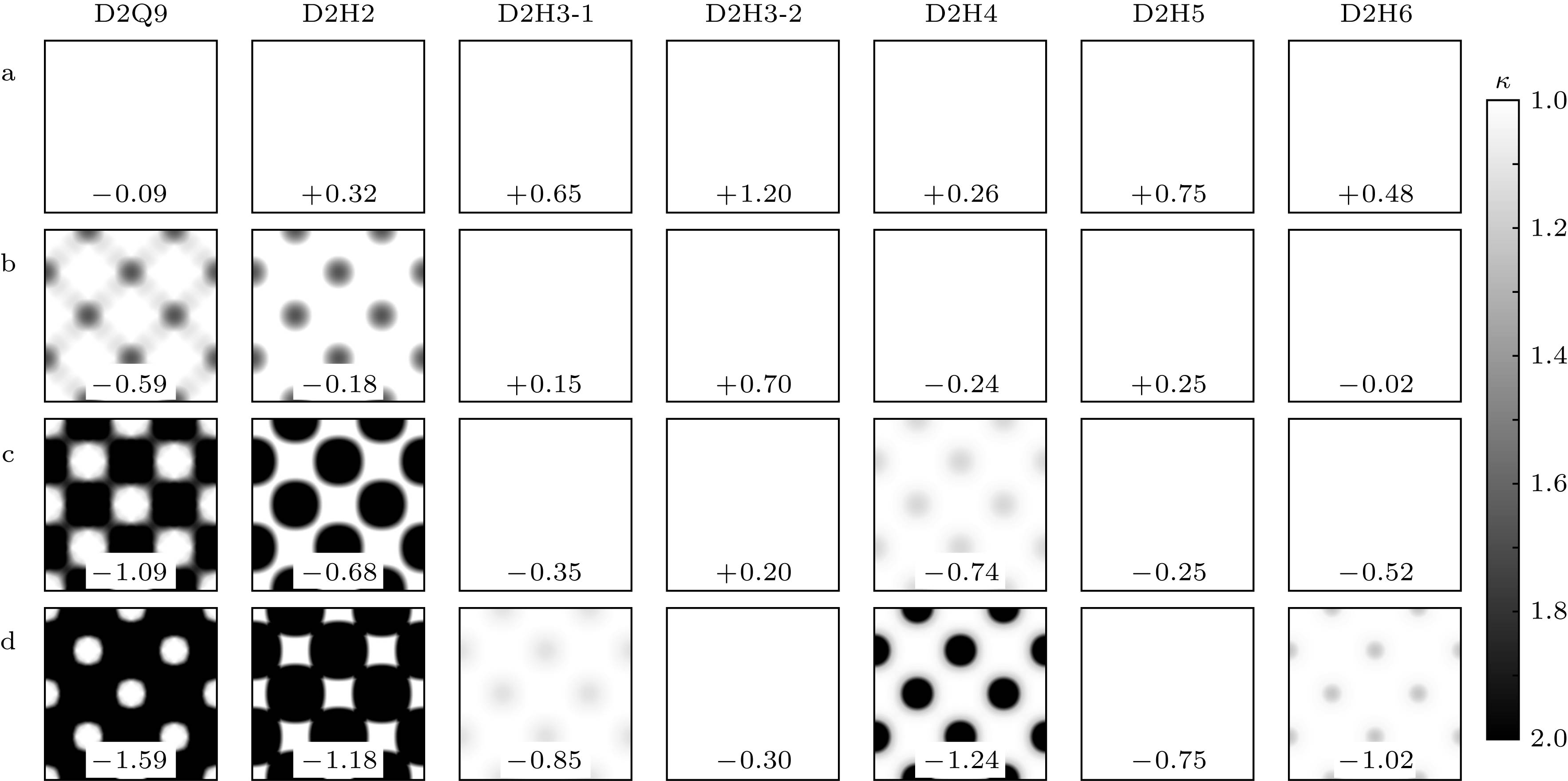
$ [0,2{\text{π}}]\times[0,2{\text{π}}] $ 内$ \kappa $ 值色阶图 图中列对应格子Boltzmann模型, 行则对应表3中计算工况; 每个色阶图上方的数值$ \Delta u $ 值, 即正值区域值$ u_{\rm pos} $ 设计计算工况$ u_{L{\rm B} ,0} $ 差值;为方便观察正值性随计算工况遭到破坏的变化过程, 图中对$ \kappa $ 值做了截断处理, 仅区别$ [1.0,2.0] $ 范围变化Fig. 2. The initial
$ \kappa $ filled contours of designed Taylor-Green vortex simulations for each lattice Boltzmann model in the fluid domain$ [0,2{\text{π}}]\times[0,2{\text{π}}] $ . Each column is a simulation set of a lattice Boltzmann model with different designed cases. Each row is a set of a simulation case with different lattice Boltzmann models. The values in the contour panels are the values of$ \Delta u $ , i.e. the difference between the$ u_{\rm pos} $ and the designed$ u_{L{\rm B} ,0} $ . For the sake of identifying the positivity violation process of a lattice Boltzmann model, the filled contours truncate the range of$ \kappa $ , limiting into$ [1.0,2.0] $ .图 3 Taylor-Green涡半衰时刻
$ t = 3.4657359\; \rm{s} $ ,$ [0.3775,0.6225]{\text{π}} \times[0.3775,0.6225]{\text{π}} $ 流域内, 不同计算工况下理论解(Theoretical) 与各格子Boltzmann模型的速度平方和$ U^2 $ 等高线图; 图中列对应格子Boltzmann模型, 行则对应表3中计算工况Fig. 3. The
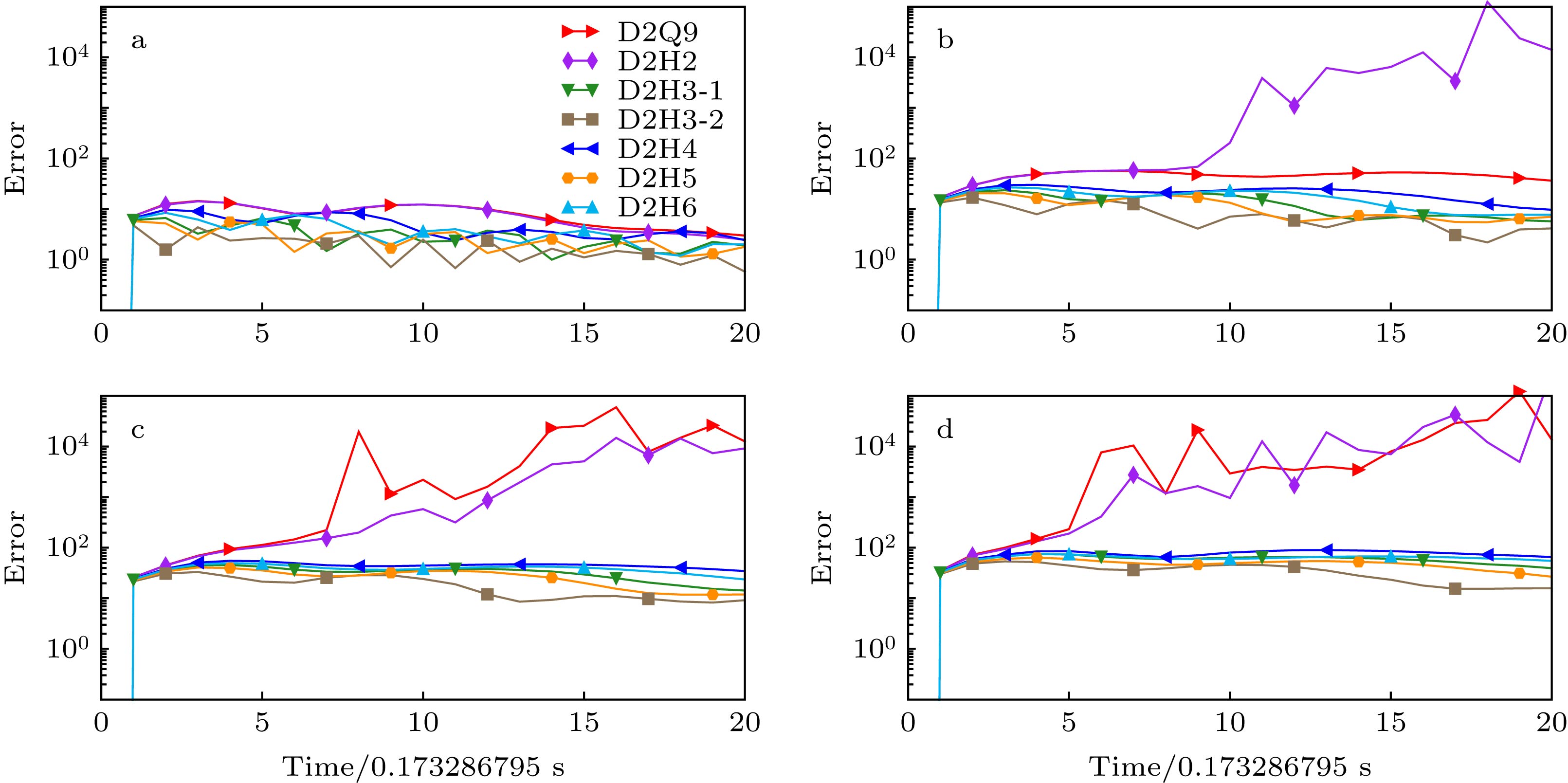
$ U^2 $ contour lines of Taylor-Green vortex in fluid domain$ [0.3775,0.6225]{\text{π}} \times[0.3775,0.6225]{\text{π}} $ at half-value decay time$ t = 3.4657359 \; \rm{s} $ , including the theoretical solution (denoted as “Theoretical”) and the numerical results of lattice Boltzmann models. Each column is a set of simulations under the designed cases. Each row is a set of simulations under selected lattice Boltzmann models including the theoretical solution.图 4 各Taylor-Green涡设计计算工况下, 各格子Boltzmann模型计算误差随时间演变, 图中标号a, b, c, d分别对应表3各设计计算工况; 为方便表示, 图中横坐标单位为
$ 0.173286795\; \rm{s} $ Fig. 4. The error evolution of each simulation. The panel a, b, c, d renders each designed case in Table 3 respectively. For the sake of rendering, the unit of the time axis is scaled as 0.173286795 s.
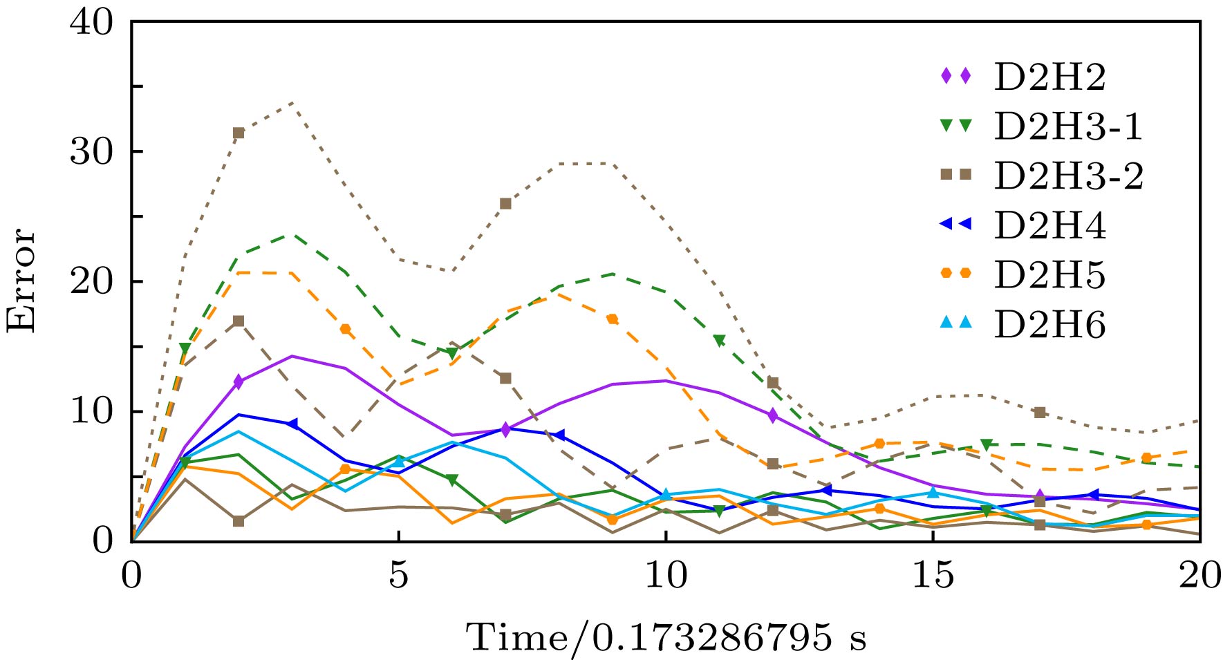
图 5 Taylor-Green涡设计计算工况下,
$ \Delta u $ 值为正值的各格子Boltzmann模型数值模拟误差对比. 图中实线, 虚线和虚点线分别为工况a, b, c (见表3)结果, 离散模型则用颜色和符号标注. 为方便表示, 图中横坐标单位为0.173286795 sFig. 5. The error comparison of Taylor-Green vortex simulations with postive value of
$ \Delta u $ . The designed configurations of Taylor-Green vortex are denoted with line styles, in which the solid, dashed and dash-dotted line indicates case a, b and c in Table 3 respectively, meanwhile the lattice Boltzmann models are labeled with line colors and markers. For the sake of rendering, the unit of the time axis is scaled as 0.173286795 s.图 6 Taylor-Green涡数值模拟误差与
$ \Delta u $ 值相关性分析 (a)对比了$ \Delta u $ 接近的D2H4模型a, b, c工况与D2H5模型b, c, d工况计算误差; (b)对比了$ \Delta u $ 在$ -0.30 $ 附近所有数值模拟计算误差. 所有图中均保留了D2H3-2模型在a, b, c, d工况下的计算误差作为参照. 曲线上标注值为该数值模拟的$ \Delta u $ 值. 图中a, b, c, d工况分别用实线, 虚线, 虚点线及点线标注, 而离散模型则用颜色和符号标注. 为方便表示, 图中横坐标单位为0.173286795 sFig. 6. The numerical performance of Taylor-Green vortex simulations vs the value of
$ \Delta u $ . Panel a plots the numerical errors of model D2H4 under case a, b, c and model D2H5 under case b, c, d, which possess close value of$ \Delta u $ respectively. Panel b plots the numerical errors of simulations with a value of$ \Delta u $ around$ -0.30 $ . The numbers labeled on the curves are their values of$ \Delta u $ . The simulation configurations are denoted with line style, in which solid, dashed, dash-dotted and dotted line indicates case a, b, c and d respectively, meanwhile the lattice Boltzmann models are labeled with line colors and markers. In all panels, the results of model D2H3-2 with four designed configurations are plotted for a reference. The designed configurations of Taylor-Green vortex are denoted with line styles, in which the solid, dashed, dash-dotted and dotted line indicates case a, b, c and d in Table 3 respectively, meanwhile the lattice Boltzmann models are labeled with line colors and markers. For the sake of rendering, the unit of the time axis is scaled as 0.173286795 s.图 7 Taylor-Green涡数值模拟误差与初始
$ \kappa $ 值相关性分析. 图中对比了在$ \Delta u $ 值为负情况下, 初始$ \kappa $ 值偏离$ 1 $ 幅值可忽略的算例计算误差, 包括模型D2H3-1工况c, 模型D2H3-2工况d, 模型D2H4工况b, 模型D2H5工况c, d和模型D2H6工况b, c. 图中均保留了D2H3-2模型在a, b, c, d工况下的计算误差作为参照. 曲线上标注值为该数值模拟的$ \Delta u $ 值. 图中a, b, c, d工况分别用实线, 虚线, 虚点线及点线标注, 而离散模型则用颜色和符号标注. 为方便表示, 图中横坐标单位为0.173286795 sFig. 7. The numerical performance of Taylor-Green vortex simulations vs initial
$ \kappa $ . The error evolutions of numerical simulations with negative values of$ \Delta u $ but negligible departure of initial$ \kappa $ from$ 1 $ are plotted, including model D2H3-1 under case c, model D2H3-2 under case d, model D2H4 under case b, model D2H5 under case c,d and model D2H6 under case b, c. The results of model D2H3-2 with four designed configurations are also plotted for a reference. The designed configurations of Taylor-Green vortex are denoted with line styles, in which the solid, dashed and dash-dotted line indicates case a, b and c in Table 3 respectively, meanwhile the lattice Boltzmann models are labeled with line colors and markers. For the sake of rendering, the unit of the time axis is scaled as 0.173286795 s.表 1 前五阶物理Hermite多项式
Table 1. The first five physicists′ Hermite polynomials.
Hermite 多项式阶数
The degree of Hermite polynomial多项式表达式
Hermite polynomial0 ${ { H}_0}\left( x \right) = 1$ 1 ${ { H}_1}\left( x \right) = 2x$ 2 ${ { H}_2}\left( x \right) = 4x^2-2$ 3 ${ { H}_3}\left( x \right) = 8x^3-12x$ 4 ${ {H}_4}\left( x \right) = 16x^4-48x^2+12$ 表 2 格子Boltzmann离散模型. 为方便展示, 表格罗列的是用于对应构造高阶模型的一维模型参数. 实际计算中需根据(9)式和(10)式对表格中的参数进行张量构造. 另外需注意的是表格中罗列的是网格常数c, 其与格子声速
$ c_{\rm s} $ 存在如下换算关系$ c = 1/\sqrt{2}c_{\rm s} $ Table 2. Discrete model description of lattice Boltzmann method. For the seeking of space saving, the parameters illustrated in this table are of the corresponding unidimensional models. In numerical implementations, they require tensor product illuminated in Eq. (9) and Eq. (10). It should be noted that the table lists the lattice constant c instead of the lattice sonic speed
$ c_{\rm s} $ , which can be expressed as$ c = 1/\sqrt{2}c_{\rm s} $ .Model name Discrete velocityset {$v_\alpha$} Lattice constant c Weights {${w}_\alpha$} D2H2 {$0, \pm 1$} $1.2247\times10^0$ {$6.6667\times10^{-1}$, 1.6667$\times10^{-1}$} D2H3-1 {$0, \pm 1, \pm 3$} $5.5343\times10^{-1}$ {$7.4464\times10^{-2}$, $4.1859\times10^{-1}$, $4.4182\times10^{-2}$} D2H3-2 {$0, \pm 2, \pm 5$} $3.4420\times10^{-1}$ {$3.1044\times10^{-1}$, $3.0997\times10^{-1}$, $3.4812\times10^{-2}$} D2H4 {$0, \pm 1, \pm 2, \pm 3$} $8.4639\times10^{-1}$ {$4.7667\times10^{-1}$, $2.3391\times10^{-1}$, $2.6938\times10^{-2}$, $8.1213\times10^{-4}$} D2H5 {$0, \pm 1, \pm 2, \pm 3, \pm 5$} $4.7940\times10^{-1}$ {$1.6724\times10^{-1}$, $3.0315\times10^{-1}$, $5.3303\times10^{-2}$, $5.7922\times10^{-2}$, $2.0013\times10^{-3}$} D2H6 {$0, \pm 1, \pm 2, \pm 3, \pm 4, \pm 5$} $6.8590\times10^{-1}$ {$3.8694\times10^{-1}$, $2.4178\times10^{-1}$, $5.8922\times10^{-2}$, $5.6153\times10^{-3}$, $2.0652\times10^{-4}$, $3.2745\times10^{-6}$} 表 3 算例设计
Table 3. Case design for lattice Boltzmann method
Case name Step time/s $u_{L{\rm B} ,0}$ a $1.570796\times10^{-2}$ 0.5 b $3.141593\times10^{-2}$ 1.0 c $4.712389\times10^{-2}$ 1.5 d $6.283185\times10^{-2}$ 2.0 -
[1] Ammar S, Pernaudat G, Trepanier J 2017 J. Comput. Phys. 343 73
 Google Scholar
[2] Li Q, Luo K H, Kang Q J, He Y L, Chen Q, Liu Q 2016 Prog. Energ. Combust. 52 62
 Google Scholar
[3] Shan X W 2010 Phys. Rev. E 81 045701
 Google Scholar
[4] Shan X W, Chen H D 1993 Phys. Rev. E 47 1815
 Google Scholar
[5] Sheikholeslami M, Gorji-Bandpy M, Ganji D D 2014 Powder Technol. 254 82
 Google Scholar
[6] Zhang X L, Xiao L Z, Shan X W, Guo L 2014 Sci. Rep. 4 4843
[7] Shan X W 2011 IMA J. Appl. Math. 76 650
 Google Scholar
[8] Kang Q J, Zhang D X, Chen S Y, He X Y 2002 Phys. Rev. E 65 036318
 Google Scholar
[9] Mountrakis L, Lorenz E, Malaspinas O, Alowayyed S, Chopard B, Hoekstra A G 2015 J. Comput. Sci. 9 45
 Google Scholar
[10] Ladd A J C, Verberg R 2001 J. Stat. Phys. 104 1191
 Google Scholar
[11] Chopard B, Ouared R, Deutsch A, Hatzikirou H, Wolf-Gladrow D 2010 Acta Biotheor. 58 329
 Google Scholar
[12] Hirabayashi M, Ohta M, Rjfenacht D A, Chopard B 2003 Phys. Rev. E 68 021918
 Google Scholar
[13] Latt J, Chopard B 2007 Int. J. Mod. Phys. C 18 619
 Google Scholar
[14] Yu H D, Luo L S, Girimaji S S 2006 Comput. Fluids 35 957
 Google Scholar
[15] Yu H D, Girimaji S S, Luo L S 2005 J. Comput. Phys. 209 599
 Google Scholar
[16] He X Y, Chen S Y, Doolen G D 1998 J. Comput. Phys. 146 282
 Google Scholar
[17] He X Y, Luo L S 1997 Phys. Rev. E 56 6811
 Google Scholar
[18] Ye H F, Kuang B, Yang Y H 2019 Chin. Phys. B 28 014701
 Google Scholar
[19] Dellar P J 2014 J. Comput. Phys. 259 270
 Google Scholar
[20] Nie X B, Shan X W, Chen H D 2008 EPL-Europhys. Lett. 81 34005
 Google Scholar
[21] Hazi G, Kavran P 2006 J. Phys. A 39 3127
 Google Scholar
[22] Shan X W 2016 J. Comput. Sci. 17 475
 Google Scholar
[23] Shan X W 2010 Phys. Rev. E 81 036702
 Google Scholar
[24] Shim J W 2013 Phys. Rev. E 87 013312
 Google Scholar
[25] Ye H F, Gan Z C, Kuang B, Yang Y H 2019 Chin. Phys. B 28 054702
 Google Scholar
[26] Shan X W, He X Y 1998 Phys. Rev. Lett. 80 65
 Google Scholar
计量
- 文章访问数: 9209
- PDF下载量: 43
- 被引次数: 0


 下载:
下载:


