


-
The incompressible Navier-Stokes equations (INSE) are the basic governing equations of fluid dynamics, and their numerical solutions are of great significance. In this review paper, we first recollect some classical projection methods and their relatives in the past 50 years and then fully explain the recent fourth-order projection method called GePUP [Zhang Q
2016 J. Sci. Comput. 67 1134 ]. Based on a generic projection operator and the UPPE formulation of the INSE [Liu J G, Liu J, Pego R L2007 Comm. Pure Appl. Math. 60 1443 ], we derive the GePUP equations, which retain the advantage of UPPE that the velocity divergence is governed by a heat equation and is thus well under control. In comparison with UPPE, the GePUP formulation is advantageous in three aspects: (1) its derivation depends on none of the properties of the Leray-Helmholtz projection; (2) the evolutionary velocity can be divergent, thus it is directly applicable to numerical calculations with nonzero velocity divergence; (3) the Leray-Helmholtz projection does appear on the right-hand sides of the governing equations, thus making it transparent to analyze the accuracy and stability issues raised by numerically approximating the Leray-Helmholtz projection. As the most appealing feature of GePUP, temporal integration and spatial discretization are completely decoupled and can be treated as black boxes, so that the user can choose his favorite methods for the two parts to form his own GePUP method. In particular, high-order accuracy in time can be easily obtained since no internal details of the ODE solver are needed. The flexibility in time makes the GePUP method applicable to both low-Reynolds-number flow and high-Reynolds-number flow. The flexibility in space makes the GePUP method applicable to both rectangular boxes and irregular domains. The numerical results and elementary analysis show that the fourth-order GePUP method may be much more accurate and efficient than classical second-order projection methods by many orders of magnitude.-
Keywords:
- incompressible Navier-Stokes equations /
- projection methods /
- fourth-order accuracy both in time and in space /
- no-slip boundary conditions /
- generic projection /
- pressure Poisson equation
[1] Smale S 1998 Mathematical Intelligencer 20 7
 Google Scholar
[2] Devlin K 2005 The Millennium Problems: the Seven Greatest Unsolved Mathematical Puzzles of Our Time (Granta Books) pp103−136
[3] Carlson J, Jaffe A, Wiles A, Editors 2006 The Millennium Prize Problems (American Mathematical Society) pp57−67
[4] Zhang Q 2014 Appl. Numer. Math. 77 16
Google Scholar
[5] Zhang Q 2016 J. Sci. Comput. 67 1134
Google Scholar
[6] Bell J B, Colella P, Glaz H M 1989 J. Comput. Phys. 85 257
Google Scholar
[7] Martin D F, Colella P, Graves D 2008 J. Comput. Phys. 227 1863
Google Scholar
[8] Taylor M E 2011 Partial Differential Equations I. No. 115 in Applied Mathematical Sciences (2nd Ed.) (Springer) pp408−409
[9] Sanderse B, Koren B 2012 J. Comput. Phys. 231 3041
Google Scholar
[10] Griffth B E 2009 J. Comput. Phys. 228 7565
Google Scholar
[11] Benzi M, Golub G H, Liesen J 2005 Acta Numer. 14 1
Google Scholar
[12] Chorin A J 1968 Math. Comput. 22 745
Google Scholar
[13] Kim J, Moin P 1985 J. Comput. Phys. 59 308
Google Scholar
[14] Orszag S A, Israeli M, Deville M O 1986 J. Sci. Comput. 1 75
Google Scholar
[15] Weinan E, Liu J G 2003 Comm. Math. Sci. 1 317
Google Scholar
[16] Guermond J L, Minev P, Shen J 2006 Comput. Methods Appl. Mech. Engrgy 195 6011
Google Scholar
[17] Brown D L, Cortez R, Minion M L 2001 J. Comput. Phys. 168 464
Google Scholar
[18] Kleiser L, Schumann U 1980 Proceedings of the Third GAMM-Conference on Numerical Methods in Fluid Mechanics, vol. 2 of Notes on Numerical Fluid Mechanics (Springer) pp 165−173
[19] Gresho P M, Sani R L 1987 Int. J. Numer. Methods Fluids 7 1115
Google Scholar
[20] Henshaw W D 1994 J. Comput. Phys. 113 13
Google Scholar
[21] Johnston H, Liu J G 2004 J. Comput. Phys. 199 221
Google Scholar
[22] Liu J G, Liu J, Pego R L 2007 Commun. Pure Appl. Math. 60 1443
Google Scholar
[23] Liu J G, Liu J, Pego R L 2010 J. Comput. Phys. 229 3428
Google Scholar
[24] Shirokoff D, Rosales R R 2011 J. Comput. Phys. 230 8619
Google Scholar
[25] Zhang Q, Johansen H, Colella P 2012 SIAM J. Sci. Comput. 34 B179
Google Scholar
[26] Li Z, Zhang Q 2021 submitted for publication
[27] Zhang Q, Li Z 2021 submitted for publication
[28] Ascher U M, Ruuth S J, Spiteri R J 1997 Appl. Numer. Math. 25 151
Google Scholar
[29] Kennedy C A, Carpenter M H 2003 Appl. Numer. Math. 44 139
Google Scholar
[30] Briggs W L, Henson V E, McCormick S F 2000 A Multigrid Tutorial (2nd Ed.) (SIAM) pp 31−43
[31] Brandt A 1986 Appl. Math. Comput. 19 23
Google Scholar
[32] Trottenberg U, Oosterlee C, Schuller A 2001 Multigrid (Elsevier Academic Press) pp439−441
[33] Shankar P N, Deshpande M D 2000 Annu. Rev. Fluid Mech. 32 93
Google Scholar
[34] Guermond J L, Migeon C, Pineau G, Quartapelle L 2002 J. Fluid. Mech. 450 169
Google Scholar
[35] Verstappen R, Veldman A 1997 J. Eng. Math. 32 143
Google Scholar
[36] Hokpunna A, Manhart M 2010 J. Comput. Phys. 229 7545
Google Scholar
[37] Almgren A, Aspden A, Bell J B, Minion M L 2013 SIAM J. Sci. Comput. 35 B25
Google Scholar
[38] Gullbrand J 2000 An Evaluation of a Conservative Fourth Order DNS Code in Turbulent Channel Center for Turbulence Research, Stanford University
[39] Shishkina O, Wagner C 2007 Comput. Fluids 36 484
Google Scholar
[40] Knikker R 2009 Int. J. Numer. Methods Fluids 59 1063
Google Scholar
[41] Adams M, Colella P, Graves D T, Johnson J, Keen N, Ligocki T J, Martin D F, McCorquodale P, Modiano D, Schwartz P, Sternberg T, Straalen B V 2014 Chombo Software Package for AMR Applications-Design Document Lawrence Berkeley National Laboratory. LBNL-6616 E
[42] Chombo http://seesar.lbl.gov/ANAG/software.html. Version 3.2
[43] Meuer H, Strohmaier E, Dongarra J, Simon H http://www.top500.org [2020-11-25]
[44] Zhang Q, Fogelson A 2016 SIAM J. Numer. Anal. 54 530
Google Scholar
[45] Zhang Q 2018 SIAM J. Sci. Comput. 40 A3755
Google Scholar
-

图 1 面平均值和控制体平均值. 面平均值用带
$ \left\langle {\cdot} \right\rangle $ 且下标为分数的符号表示, 而控制体平均值对应下标为整数. 因此$ \left\langle {\phi} \right\rangle_{ {{i}}+\frac{1}{2} {{e}}^0} $ ,$ \left\langle {\phi} \right\rangle_{ {{i}}- {{e}}^0+\frac{1}{2} {{e}}^1} $ 和$ \left\langle {u_0} \right\rangle_{ {{i}}+\frac{3}{2} {{e}}^0 + {{e}}^1} $ 表示面平均值, 而$ \left\langle {\phi} \right\rangle_{ {{i}}} $ 是控制体平均值[5]Figure 1. Notation of face-averaged and cell-averaged values. A symbol with angled brackets denotes either a cell-averaged value if the subscript is an integer multi-index, or a face-averaged value if the subscript is a fractional multi-index. Hence
$ \left\langle {\phi} \right\rangle_{ {{i}}+\frac{1}{2} {{e}}^0} $ ,$ \left\langle {\phi} \right\rangle_{ {{i}}- {{e}}^0+\frac{1}{2} {{e}}^1} $ , and$ \left\langle {u_0} \right\rangle_{ {{i}}+\frac{3}{2} {{e}}^0 + {{e}}^1} $ are face-averaged values while$ \left\langle {\phi} \right\rangle_{ {{i}}} $ is a cell-averaged value. Horizontal and vertical hatches represent the averaging processes over a vertical cell face and a horizontal cell face, respectively. Light gray area represents averaging over a cell[5].
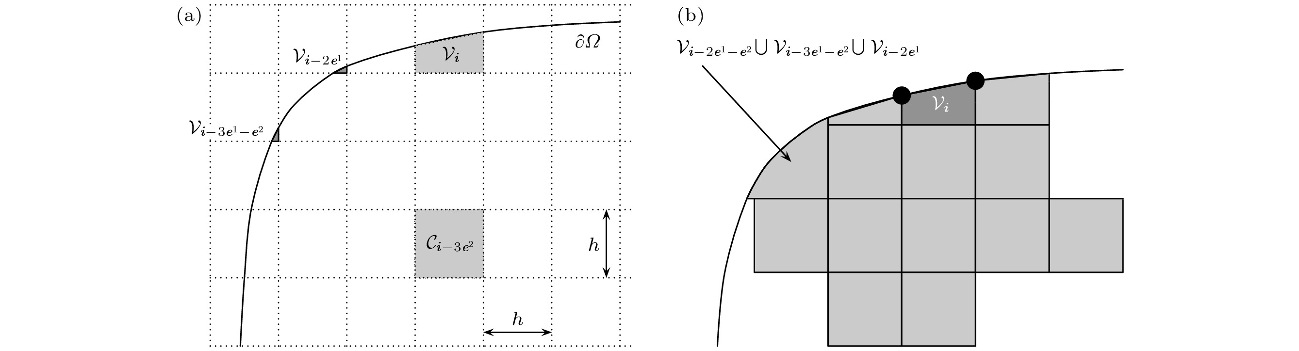

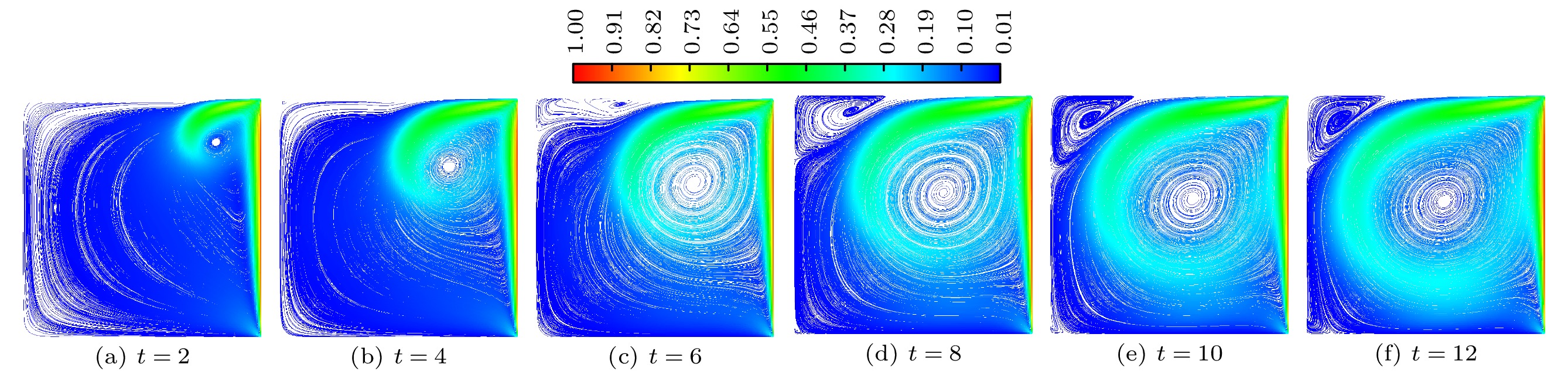
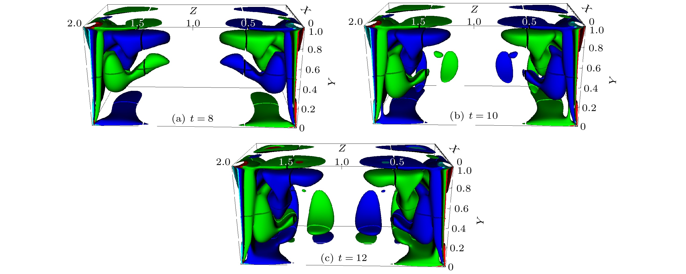
图 6 三维顶盖驱动方腔流测试中均匀网格上(
$h = {1}/{128}$ )涡量的x-分量等值面. 红色, 橙色, 蓝色和青色对应的涡量x-分量值分别为–0.50, –0.25, 0.25和0.50[5]Figure 6. Isosurfaces of the x component of the vorticity vector for the 3D lid-driven cavity test on a uniform grid with
$h = {1}/{128}$ . The values of the vorticity component for the red, orange, blue, cyan surfaces are –0.50, –0.25, 0.25, and 0.50, respectively[5].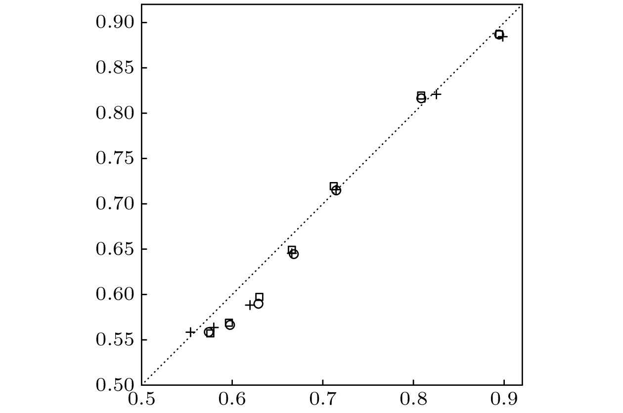
图 7 时刻
$ t = 1, 2, 4, 6, 8, 10, 12 $ 对称平面$ z = 0 $ 上主旋涡的中心位置比较. “$ \circ $ ”表示本文的数值结果(由最小化$ \|{u}\|_2 $ 得到), 而“+”和“$ \square $ ”分别是Guermond等[34]得到的实验和计算结果[5]Figure 7. A comparison of the center locations of the primary eddy in the symmetry plane
$ z = 0 $ at time instances$ t = 1, 2, 4, 6, 8, 10, 12 $ . The circles represent numerical results of this work, which are determined by minimizing the speed$ \|{u}\|_2 $ . The experimental and computational results of Guermond et. al.[34] are represented by the crosses and the squares, respectively[5].
图 8 三维顶盖驱动方腔流在时刻
$ t = 12 $ 的流速剖面图比较($h = {1}/{128}$ ). 实线表示本文的数值结果, 即$ -\frac{1}{2}u $ 和$ \frac{1}{2}v $ 分别作为$ \frac{1}{2}-y $ 和$ \frac{1}{2}-x $ 的函数. “$ \times $ ”和“$ \cdot $ ”分别表示Guermond等[34]得到的实验和计算结果[5]Figure 8. A comparison of velocity profiles for the three dimensional lid-driven cavity test (
$h = {1}/{128}$ ) at$ t = 12 $ . Solid lines represent computational results of this work, i.e.$ -\frac{1}{2}u $ as a function of$ \frac{1}{2}-y $ and$ \frac{1}{2}v $ as a function of$ \frac{1}{2}-x $ . The computational and experimental results of Guermond et. al.[34] are represented by the solid dots and crosses, respectively[5].
图 9 二维顶盖驱动方腔流测试中均匀网格上
$(h = {1}/{128})$ 的流速场Figure 9. Numerical results of the velocity field in the two dimensional lid-driven cavity test on the unit box and the rotated box with
$h = {1}/{128}$ .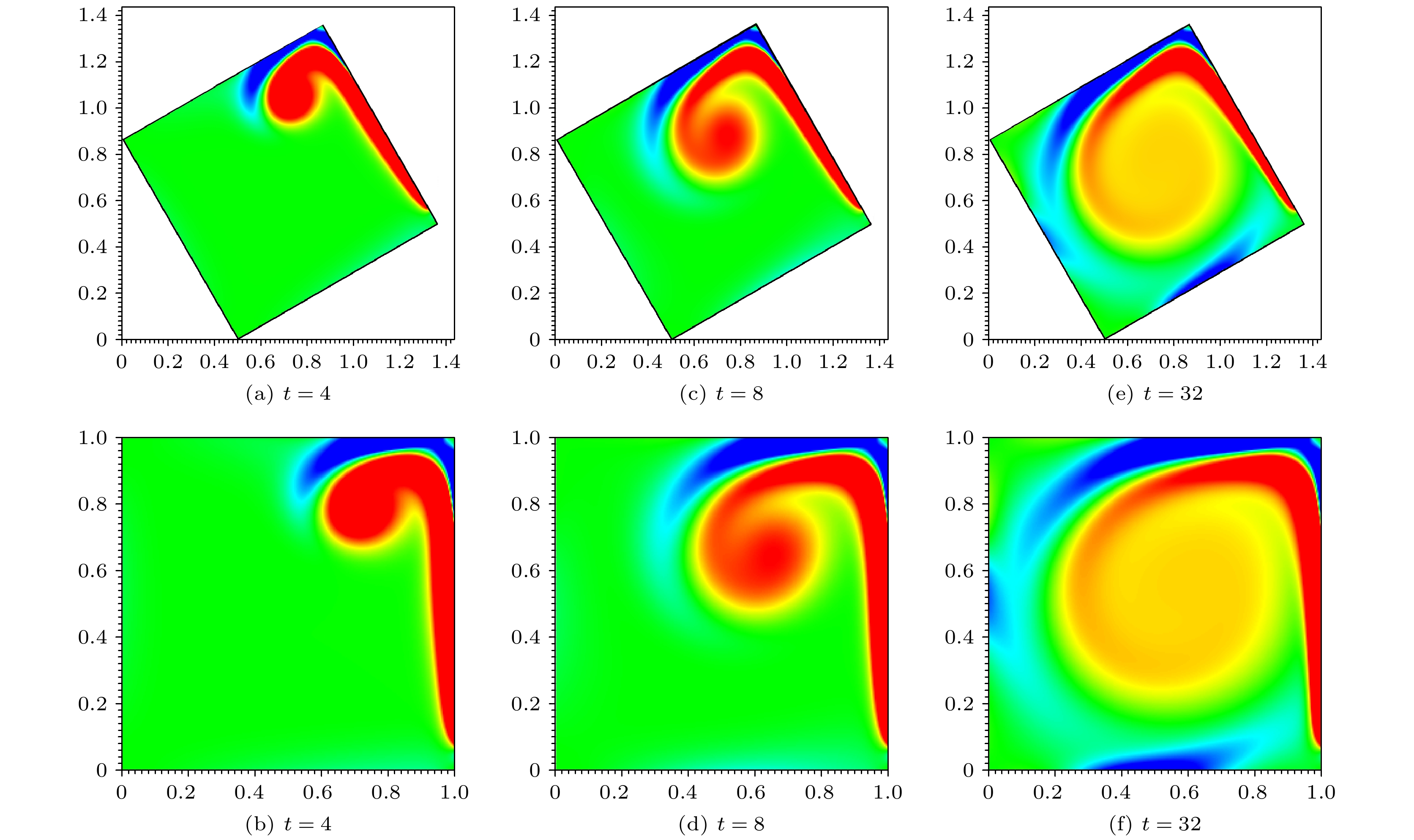
图 10 二维顶盖驱动方腔流测试中均匀网格上
$(h = {1}/{128})$ 的涡量快照Figure 10. Numerical results of the vorticity in the two dimensional lid-driven cavity test on the unit box and the rotated box with
$h = {1}/{128}$ .表 1 用GePUP-ERK算法在不规则计算域(87)上求解以(88)式和(89)式为解析解的INSE得到的误差和收敛阶. Re = 1000,
$ t_0 = 0 $ ,$ t_{\rm e} = 0.1 $ ,$ {{\textsf{Cr}}} = 0.2 $ [5]Table 1. Errors and convergence rates of GePUP-ERK for solving the INSE on the irregular domain (87) with Eq. (88) and Eq. (89) as the analytic solutions. Re = 1000,
$ t_0 = 0 $ ,$ t_{\rm e} = 0.1 $ ,$ {{\textsf{Cr}}} = 0.2 $ [5].h ${1}/{32}$ Rate ${1}/{64}$ Rate $1/{128}$ Rate $1/{256}$ ${u}$ $ L_{\infty} $ 2.63 × 10⁻⁴ 3.94 1.71 × 10⁻⁵ 3.98 1.08 × 10⁻⁶ 4.00 6.78 × 10⁻⁸ $ {u} $ $ L_1 $ 1.63 × 10⁻⁴ 3.87 1.12 × 10⁻⁵ 3.97 7.14 × 10⁻⁷ 3.99 4.48 × 10⁻⁸ $ {u} $ $ L_2 $ 1.49 × 10⁻⁴ 3.89 1.01 × 10⁻⁵ 3.98 6.38 × 10⁻⁷ 4.00 4.00 × 10⁻⁸ p $ L_{\infty} $ 1.63 × 10⁻³ 3.99 1.02 × 10⁻⁴ 4.00 6.39 × 10⁻⁶ 4.01 3.97 × 10⁻⁷ p $ L_1 $ 3.26 × 10⁻⁴ 4.00 2.04 × 10⁻⁵ 4.03 1.25 × 10⁻⁶ 3.97 7.97 × 10⁻⁸ p $ L_2 $ 4.60 × 10⁻⁴ 3.99 2.89 × 10⁻⁵ 4.01 1.80 × 10⁻⁶ 3.99 1.13 × 10⁻⁷  DownLoad: CSV
表 2 不同的测试中为了达到同样的
$ L_2 $ 流速计算精度$ \epsilon $ , GePUP-IMEX相对于MCG[7]的性能加速比$ S_{4 |2} $ [5]Table 2. The speedup
$ S_{4 |2} $ of GePUP-IMEX over MCG[7] for achieving the same$ L_2 $ accuracy$ \epsilon $ of the velocity[5].$ S_{4 |2} $ $ \epsilon = 10^{-4} $ $ \epsilon = 10^{-6} $ $ \epsilon = 10^{-8} $ $ \epsilon = 10^{-10} $ 单涡量测试, Re = $ 2\times 10^4 $ 1.73 5.50 × 101 1.73 × 10³ 5.47 × 10⁴ 二维粘盒测试, Re = $ 10^4 $ 5.03 1.59 × 10² 5.03 × 10³ 1.59 × 10⁵ 二维粘盒测试, Re = 100 1.26 × 101 4.00 × 10² 1.26 × 10⁴ 3.98 × 10⁵ 三维粘盒测试, Re = $ 10^4 $ 8.65 × 101 8.65 × 10³ 8.65 × 10⁵ 8.65 × 10⁷ 三维粘盒测试, Re = 100 4.24 × 101 4.24 × 10³ 4.24 × 10⁵ 4.24 × 10⁷
DownLoad: CSV
表 3 不同的测试中为了达到同样的
$ L_{\infty} $ 涡量计算精度$ \epsilon $ , GePUP-IMEX相对于MCG[7]的性能加速比$ S_{3 |1} $ [5]Table 3. The speedup
$ S_{3 |1} $ of GePUP-IMEX over MCG[7] for achieving the same$ L_{\infty} $ accuracy$ \epsilon $ of the vorticity[5].$ S_{3 |1} $ $ \epsilon = 10^{-2} $ $ \epsilon = 10^{-3} $ $ \epsilon = 10^{-4} $ $ \epsilon = 10^{-5} $ 单涡量测试, Re = $ 2\times 10^4 $ 1.89 × 10⁴ 1.89 × 10⁶ 1.89 × 10⁸ 1.89 × 10¹⁰ 二维粘盒测试, Re = $ 10^4 $ 2.30 × 10⁵ 2.30 × 10⁷ 2.30 × 10⁹ 2.30 × 10¹¹ 三维粘盒测试, Re = $ 10^4 $ 3.66 × 10⁷ 1.70 × 10¹⁰ 7.88 × 10¹² 3.66 × 10¹⁵
DownLoad: CSV
-
[1] Smale S 1998 Mathematical Intelligencer 20 7
Google Scholar
[2] Devlin K 2005 The Millennium Problems: the Seven Greatest Unsolved Mathematical Puzzles of Our Time (Granta Books) pp103−136
[3] Carlson J, Jaffe A, Wiles A, Editors 2006 The Millennium Prize Problems (American Mathematical Society) pp57−67
[4] Zhang Q 2014 Appl. Numer. Math. 77 16
Google Scholar
[5] Zhang Q 2016 J. Sci. Comput. 67 1134
Google Scholar
[6] Bell J B, Colella P, Glaz H M 1989 J. Comput. Phys. 85 257
Google Scholar
[7] Martin D F, Colella P, Graves D 2008 J. Comput. Phys. 227 1863
Google Scholar
[8] Taylor M E 2011 Partial Differential Equations I. No. 115 in Applied Mathematical Sciences (2nd Ed.) (Springer) pp408−409
[9] Sanderse B, Koren B 2012 J. Comput. Phys. 231 3041
Google Scholar
[10] Griffth B E 2009 J. Comput. Phys. 228 7565
Google Scholar
[11] Benzi M, Golub G H, Liesen J 2005 Acta Numer. 14 1
Google Scholar
[12] Chorin A J 1968 Math. Comput. 22 745
Google Scholar
[13] Kim J, Moin P 1985 J. Comput. Phys. 59 308
Google Scholar
[14] Orszag S A, Israeli M, Deville M O 1986 J. Sci. Comput. 1 75
Google Scholar
[15] Weinan E, Liu J G 2003 Comm. Math. Sci. 1 317
Google Scholar
[16] Guermond J L, Minev P, Shen J 2006 Comput. Methods Appl. Mech. Engrgy 195 6011
Google Scholar
[17] Brown D L, Cortez R, Minion M L 2001 J. Comput. Phys. 168 464
Google Scholar
[18] Kleiser L, Schumann U 1980 Proceedings of the Third GAMM-Conference on Numerical Methods in Fluid Mechanics, vol. 2 of Notes on Numerical Fluid Mechanics (Springer) pp 165−173
[19] Gresho P M, Sani R L 1987 Int. J. Numer. Methods Fluids 7 1115
Google Scholar
[20] Henshaw W D 1994 J. Comput. Phys. 113 13
Google Scholar
[21] Johnston H, Liu J G 2004 J. Comput. Phys. 199 221
Google Scholar
[22] Liu J G, Liu J, Pego R L 2007 Commun. Pure Appl. Math. 60 1443
Google Scholar
[23] Liu J G, Liu J, Pego R L 2010 J. Comput. Phys. 229 3428
Google Scholar
[24] Shirokoff D, Rosales R R 2011 J. Comput. Phys. 230 8619
Google Scholar
[25] Zhang Q, Johansen H, Colella P 2012 SIAM J. Sci. Comput. 34 B179
Google Scholar
[26] Li Z, Zhang Q 2021 submitted for publication
[27] Zhang Q, Li Z 2021 submitted for publication
[28] Ascher U M, Ruuth S J, Spiteri R J 1997 Appl. Numer. Math. 25 151
Google Scholar
[29] Kennedy C A, Carpenter M H 2003 Appl. Numer. Math. 44 139
Google Scholar
[30] Briggs W L, Henson V E, McCormick S F 2000 A Multigrid Tutorial (2nd Ed.) (SIAM) pp 31−43
[31] Brandt A 1986 Appl. Math. Comput. 19 23
Google Scholar
[32] Trottenberg U, Oosterlee C, Schuller A 2001 Multigrid (Elsevier Academic Press) pp439−441
[33] Shankar P N, Deshpande M D 2000 Annu. Rev. Fluid Mech. 32 93
Google Scholar
[34] Guermond J L, Migeon C, Pineau G, Quartapelle L 2002 J. Fluid. Mech. 450 169
Google Scholar
[35] Verstappen R, Veldman A 1997 J. Eng. Math. 32 143
Google Scholar
[36] Hokpunna A, Manhart M 2010 J. Comput. Phys. 229 7545
Google Scholar
[37] Almgren A, Aspden A, Bell J B, Minion M L 2013 SIAM J. Sci. Comput. 35 B25
Google Scholar
[38] Gullbrand J 2000 An Evaluation of a Conservative Fourth Order DNS Code in Turbulent Channel Center for Turbulence Research, Stanford University
[39] Shishkina O, Wagner C 2007 Comput. Fluids 36 484
Google Scholar
[40] Knikker R 2009 Int. J. Numer. Methods Fluids 59 1063
Google Scholar
[41] Adams M, Colella P, Graves D T, Johnson J, Keen N, Ligocki T J, Martin D F, McCorquodale P, Modiano D, Schwartz P, Sternberg T, Straalen B V 2014 Chombo Software Package for AMR Applications-Design Document Lawrence Berkeley National Laboratory. LBNL-6616 E
[42] Chombo http://seesar.lbl.gov/ANAG/software.html. Version 3.2
[43] Meuer H, Strohmaier E, Dongarra J, Simon H http://www.top500.org [2020-11-25]
[44] Zhang Q, Fogelson A 2016 SIAM J. Numer. Anal. 54 530
Google Scholar
[45] Zhang Q 2018 SIAM J. Sci. Comput. 40 A3755
Google Scholar


 DownLoad:


Catalog
Metrics
- Abstract views: 7558
- PDF Downloads: 278
- Cited By: 0
