-
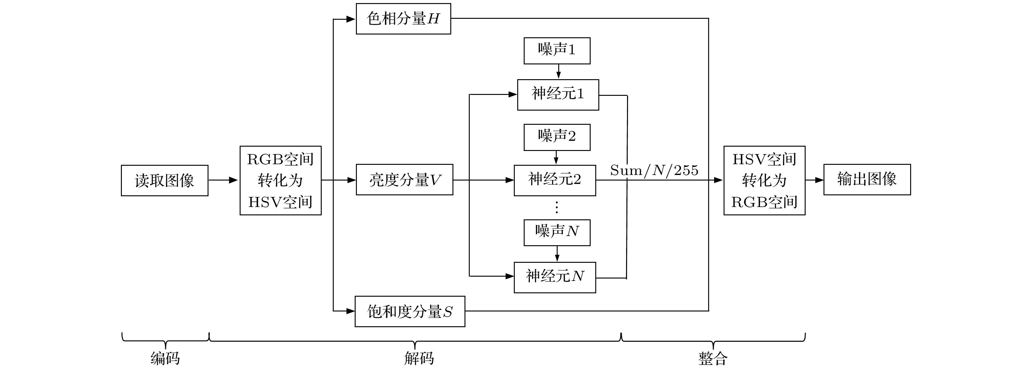
Our aim is to present an interpretable algorithm for enhancing low-illuminance color image based on the principle of stochastic resonance and the fundamental biophysical process of human brain perceiving object color. To this end, the phenomenon of stochastic resonance in a conductance-based integrate-and-fire neuronal network is first explored, with the effect of firing threshold, synaptic weight and the population size on the signal-to-noise ratio revealed, and the firing threshold is recognized as the key parameter for the resonance effects. And then, a color image enhancement algorithm, where the peak signal-to-noise ratio and the natural image quality evaluator are adopted as quantifying indexes, is developed by combining the stochastic spiking neuronal network and the involved biophysical process relating to visual perception. Note that the enhanced image is aperiodic, thus in order to optimize the performance of the algorithm, an illuminance distribution based threshold strategy is given by us for the first time. The numerical tests show that the algorithm has good enhancement performance and stability. We wish this algorithm could be applied to relevant signal processing fields such as military detection and medical image preprocessing.
-
Keywords:
- color image enhancement /
- integrate-and-fire neuronal network /
- stochastic resonance /
- biophysical interpretability
[1] Gonzalez C R, Woods R E 2002 Digital Image Processing (2nd Ed.) (New Jersey: Prentice Hall) pp88–108
[2] Kwong R H, Johnston E W 1992 IEEE Trans. Signal Process. 40 1633
 Google Scholar
[3] Dai Q, Pu Y F, Rahman Z, Aamir Z 2019 Symmetry Basel 11 574
 Google Scholar
[4] Benzi R, Sutera A, Vulpiani, A 1981 J. Phys. A-Math. Gen. 14 453
 Google Scholar
[5] Gammaitoni L, Hanggi P, Jung P, Marchesoni F 1998 Rev. Mod. Phys. 70 223
 Google Scholar
[6] Simonotto E, Riani M, Seife C, Roberts M, Twitty J, Moss F 1997 Phys. Rev. Lett. 78 1186
 Google Scholar
[7] Sasaki H, Sakane S, Ishida T, Todorokihara M, Kitamura T, Aoki R 2008 Behav. Brain. Res. 193 152
 Google Scholar
[8] Yang T 1998 Phys. Lett. A 245 79
 Google Scholar
[9] Delahaies A, Rousseau D, Fasqueal J B, Chapeau-Blondeau F 2012 J. Opt. Soc. Am. A: 29 1211
[10] Jha R K, Chouhan R 2014 Signal Image Video Process. 8 339
 Google Scholar
[11] Dylov D V, Fleischer J W 2010 Nat. Photonics 4 323
 Google Scholar
[12] Patel A, Kosko B 2011 IEEE Trans. Signal Process. 59 488
 Google Scholar
[13] Itzcovich E, Riani M, Sannita W G 2017 Sci. Rep. 7 12840
 Google Scholar
[14] Van-der-Groen O, Tang M F, Wenderoth N, Mattingley J B, Jeff B 2018 PLoS Comput. Biol. 14 1
[15] Nnoli U 2019 Optik 195 163111
 Google Scholar
[16] Kang Y M, Xu J X, Xie Y 2005 Phys. Rev. E 72 021902
 Google Scholar
[17] Yu Y G, Richard R D, Lee T S 2005 Phys. Rev. Lett. 94 108103
 Google Scholar
[18] Ashok P, Bart K 2008 IEEE Trans. Neural Networks 19 1993
[19] Purves D 2011 Brains: How They Seem to Work (New Jersey : Financial Times Press Science) pp30–47
[20] Li Z P 2019 Curr. Opin. Neurobiol. 58 1
[21] Fu Y X, Kang Y M, Chen G R 2020 Front. Comput. Neurosci. 14 24
 Google Scholar
[22] Rolls E L, Loh M, Deco G, Winterer G 2008 Nat. Rev. Neurosci. 9 696
 Google Scholar
[23] Smith R A 1978 Siggraph Comput. Graph 12 12
 Google Scholar
[24] Lagnado L 2000 Exp. Physiol. 85 1
 Google Scholar
[25] Kang Y M, Liu R N, Mao X R 2021 Cognitive Neurodynamics 15 517
 Google Scholar
[26] Tiwari I, Phogat R, Parmananda P, Ocampo-Espindola J L, Rivera L 2016 Phys. Rev. E 94 022210
 Google Scholar
[27] Mittal A, Soundararajan R, Bovik A C 2013 IEEE Signal Process. Let. 20 209
 Google Scholar
[28] Durrant S, Kang Y M, Stocks N, Feng J F 2011 Phys. Rev. E 84 011923
 Google Scholar
[29] Faisal A A, Selen L P J, Wolpert D P 2008 Nat. Rev. Neurosci. 9 292
 Google Scholar
[30] Wilke S D, Eurich C 2001 W 10th Computational Neuroscience Meeting Monterey, USA, June, 2001 p1023
[31] Wiesenfeld K, Moss F 1995 Nature 373 33
 Google Scholar
[32] Levin J E, Miller J P 1996 Nature 380 165
 Google Scholar
[33] Stacey W C, Durand D M 2000 J. Neurosci. 83 1394
-
图 1 模型(1)的时间历程图 (a)仅含漏电项的单个神经元膜电位示意图,
${V_{{\text{re}}}}=-0.3$ ; (b)无噪声时单个神经元的膜电位演化; (c)有噪声时单个神经元的膜电位演化; (d)有噪声的单个神经元的放电序列串; (e)有噪声神经元集群的放电格栅图, 其中实心点代表当前时刻所对应的神经元有动作电位产生. 图(b)至图(e)参数:${V_{\rm th}} = 0.3$ ,${V_{\rm re}} = $ $ 0$ ,${g_{\rm{l}}} = {g_{\rm{s}}} = 1$ ,${C_m} = 1$ ,${E_{\rm syn}} = 0$ ,$\varepsilon = 0.1$ ,$ \varOmega = 1 $ ,${\tau _{{s}}} = 1$ ,${\tau _{\rm{d}}} = 0.5$ ,$N = 50$ ,$t = 100$ ; (b)$D = 0$ ; (c), (e)$D = $ $ 0.025$ Figure 1. The evolution diagram of model (1): (a)Single neuron’s potential only with leaky term,
${V_{{\text{re}}}}=-0.3$ ; (b) single neuron’s membrane potential evolution without noise; (c) single Neuron’s membrane potential evolution with noise; (d) single neuron’s spike train with noise; (e) raster plot of the network where every node denotes a spike at a corresponding time and neuron. Parameters from picture (b) to (e) are set as${V_{\rm th}} = 0.3$ ,${V_{\rm re}} = 0$ ,${g_{\rm{l}}} = {g_{\rm{s}}} = 1$ ,${C_m} = 1$ ,${E_{\rm syn}} = 0$ ,$\varepsilon = 0.1$ ,$ \varOmega = 1 $ ,${\tau _{{s}}} = 1$ ,${\tau _{\rm{d}}} = 0.5$ ,$N = 50$ ,$t = 100$ ; (b)$D = 0$ ; (c), (e)$D = 0.025$ .图 2 (a)信噪比随阈值
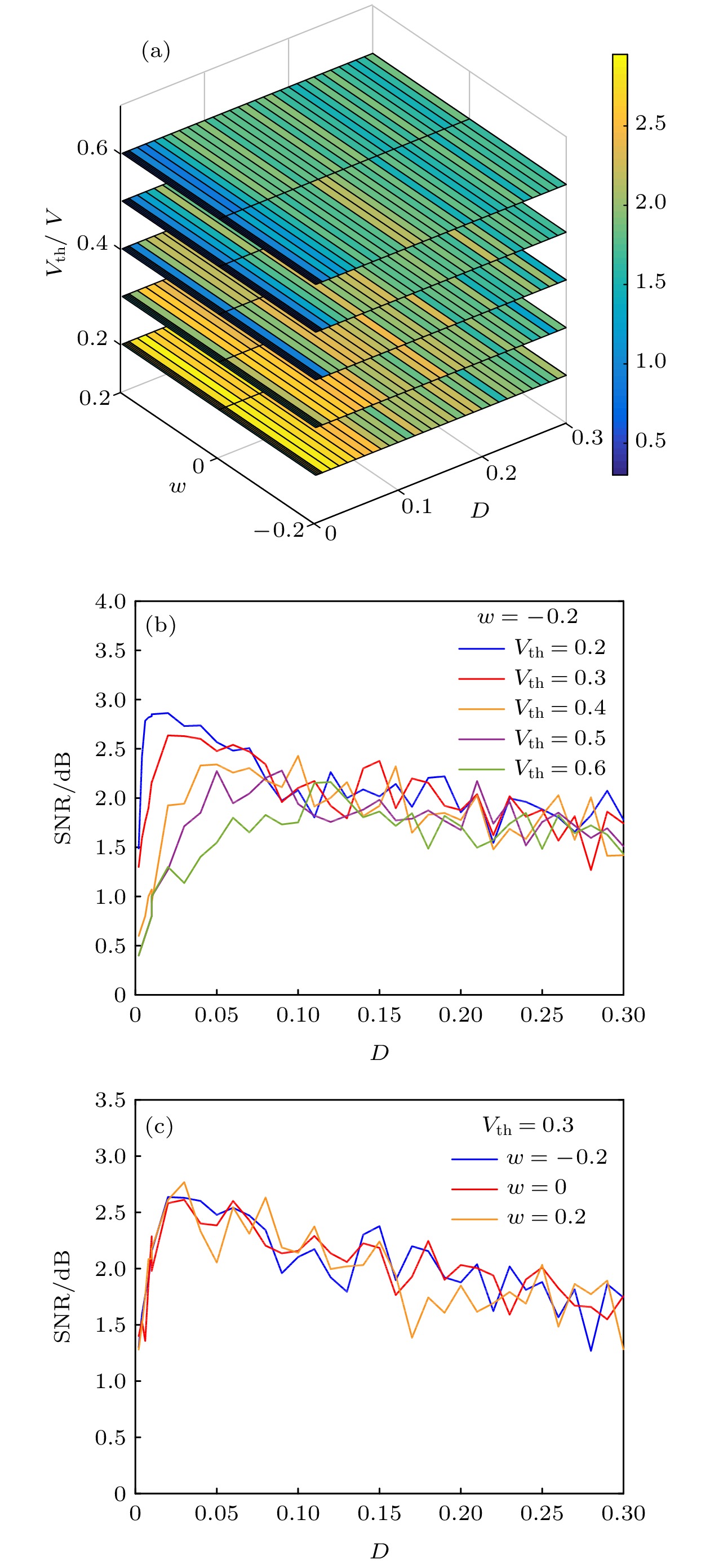
${V_{\rm th}}$ , 突触权重$w$ 变化图; (b)不同阈值信噪比变化情况; (c)不同突触权重信噪比变化情况. 参数${V_{\rm re}} = 0$ ,${g_{\rm{l}}} = {g_{\rm{s}}} = 1$ ,${C_{\rm{m}}} = 1$ ,${E_{\rm syn}} = 0$ ,$\varepsilon = 0.1$ ,$ \varOmega = 1 $ ,${\tau _{{s}}} = 1$ ,${\tau _{\rm{d}}} = 0.5$ ,$N = 5$ ,$t = 100$ Figure 2. (a) Signal-to-noise ratio for different threshold Vth and synaptic weight w; (b) signal-to-noise ratio for different threshold Vth; (c) signal-to-noise ratio for different synaptic weight w. Parameters are set as
${V_{\rm re}} = 0$ ,${g_{\rm{l}}} = {g_{\rm{s}}} = 1$ ,${C_{\rm{m}}} = 1$ ,${E_{\rm syn}} = 0$ ,$\varepsilon = 0.1$ ,$ \Omega = 1 $ ,${\tau _{{s}}} = 1$ ,${\tau _{\text{d}}} = 0.5$ ,$N = 5$ ,$t = 100$ .图 3 信噪比随神经元集群尺寸变化图, 参数
${V_{\rm th}} = 0.3$ ,$w = - 0.2$ ,${V_{\rm re}} = 0$ ,${g_{\rm{l}}} = {g_{\rm{s}}} = 1$ ,${C_{\rm{m}}} = 1$ ,${E_{\rm syn}} = 0$ ,$\varepsilon = 0.1$ ,$ \varOmega = 1 $ ,${\tau _{{s}}} = 1$ ,${\tau _{\rm{d}}} = 0.5$ ,$t = 100$ Figure 3. Signal-to-noise ratio for different quantity of neurons with
${V_{\rm th}} = 0.3$ ,$w = - 0.2$ ,${V_{\rm re}} = 0$ ,${g_{\rm{l}}} = {g_{\rm{s}}} = 1$ ,${C_{\rm{m}}} = 1$ ,${E_{\rm syn}} = 0$ ,$\varepsilon = 0.1$ ,$ \varOmega = 1 $ ,${\tau _{{s}}} = 1$ ,${\tau _{\rm{d}}} = 0.5$ ,$t = 100$ .图 6 不同神经元个数对最优增强图像质量的影响 (a)神经元个数N=50; (b)神经元个数N=300; (c)峰值信噪比(PSNR)变化曲线, 虚线代表在此噪声强度取得最优图像. 参数
${V_{{\text{th}}}} = 0.0667$ ,$w = - 0.2$ ,${V_{{\text{re}}}} = 0$ ,${g_{\text{l}}} = {g_{\text{s}}} = 1$ ,${C_{\text{m}}} = 1$ ,${E_{{\text{syn}}}} = 0$ ,${\tau _s} = 1$ ,${\tau _{\text{d}}} = 0.5$ ,$t = 100$ Figure 6. Difference caused by the size of neuron population: (a) N=50; (b) N=300; (c) peak signal-to-noise ratio(PSNR) curve, the dotted line reflects the noise density corresponds to the best enhanced picture. Parameters are set as
${V_{{\text{th}}}} = 0.0667$ ,$w = - 0.2$ ,${V_{{\text{re}}}} = 0$ ,${g_{\text{l}}} = {g_{\text{s}}} = 1$ ,${C_{\text{m}}} = 1$ ,${E_{{\text{syn}}}} = 0$ ,${\tau _s} = 1$ ,${\tau _{\text{d}}} = 0.5$ ,$t = 100$ .图 8 不同阈值下对应的最优增强图像 (a) 0.6分位点; (b) 0.95分位点; (c) 峰值信噪比变化曲线, 虚线处表示最优噪声强度. 参数
$w = - 0.2$ ,${V_{{\text{re}}}} = 0$ ,${g_{\text{l}}} = {g_{\text{s}}} = 1$ ,${C_{\text{m}}} = 1$ ,${E_{{\text{syn}}}} = 0$ ,${\tau _s} = 1$ ,${\tau _{\text{d}}} = 0.5$ ,$N = 300$ ,$t = 100$ Figure 8. Best enhanced images with different membrane potential thresholds: (a) 60 percent quantile; (b) 95 percent quantile; (c) peak signal-to-noise ratio(PSNR) curves, the dotted line reflects the noise density corresponds to the best enhanced picture. Parameters are set as
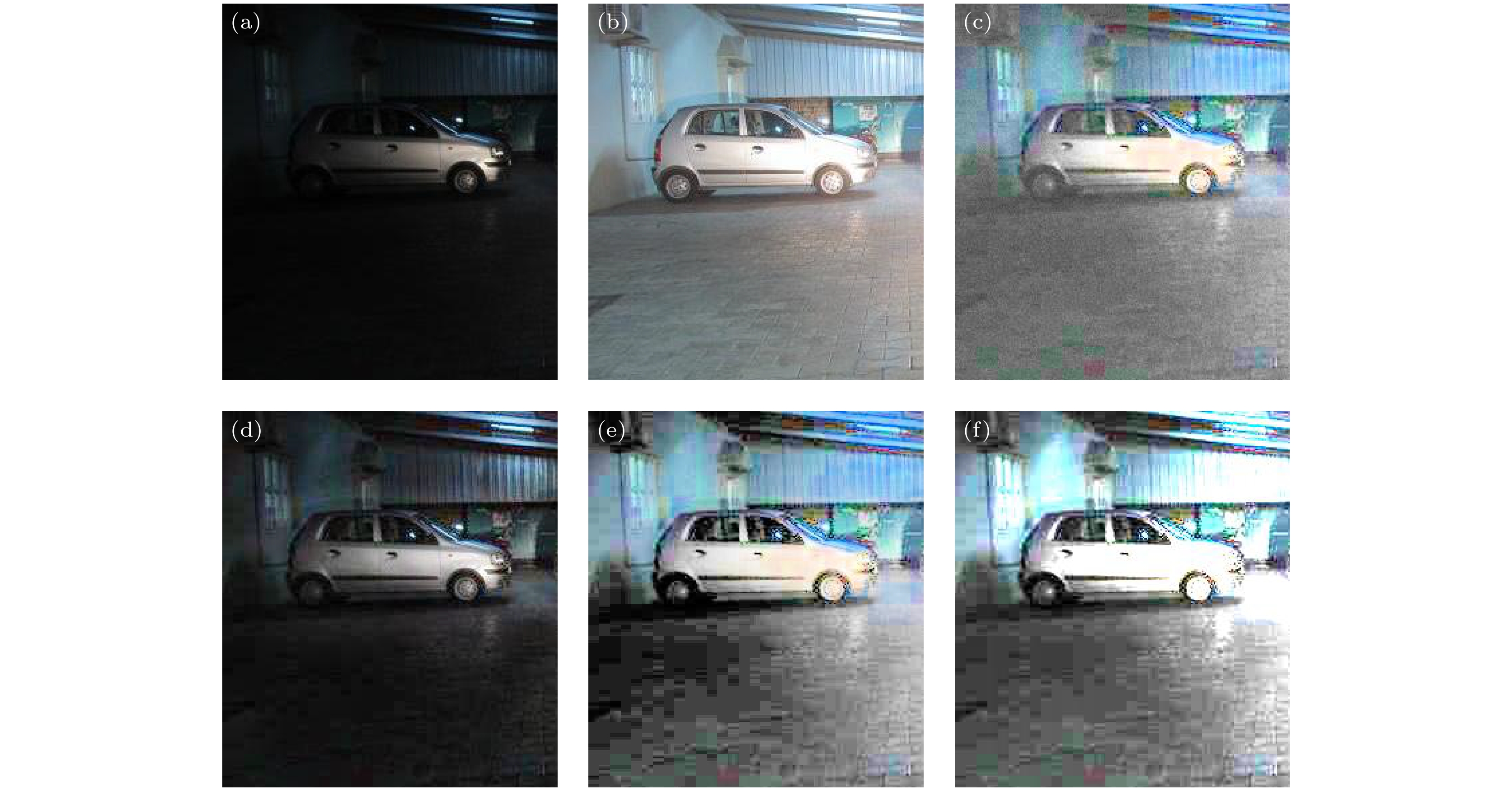
$w = - 0.2$ ,${V_{{\text{re}}}} = 0$ ,${g_{\text{l}}} = {g_{\text{s}}} = 1$ ,${C_{\text{m}}} = 1$ ,${E_{{\text{syn}}}} = 0$ ,${\tau _ s} = 1$ ,${\tau _{\text{d}}} = 0.5$ ,$N = 300$ ,$t = 100$ .图 9 图像增强结果 (a) 原始黑暗图像; (b) 原始清晰图像; (c) 本文提出的随机共振方法,
$D = 0.0035$ ,${V_{{\text{th}}}} = 0.0667$ ; (d) SSR算法; (e) HE算法; (f) SVD-DSR算法Figure 9. (a) The origin dark image; (b) the origin bright image; (c) our stochastic-resonance algorithm with
$D = 0.0035$ and${V_{{\text{th}}}} = 0.0667$ ; (d) SSR algorithm; (e) HE algorithm; (f) SVD-DSR algorithm.图 10 图像增强结果 (a) 原始黑暗图像; (b) 本文提出的随机共振方法
$D = 0.0035$ ,${V_{{\text{th}}}} = 0.11$ ; (c) SSR算法; (d) HE算法; (e) SVD-DSR算法; (f) NIQE变化图Figure 10. (a) The origin dark image; (b) our stochastic-resonance algorithm with
$D = 0.0035$ and${V_{{\text{th}}}} = 0.11$ ; (c) SSR algorithm; (d) HE algorithm; (e) SVD-DSR algorithm; (f) NIQE under different noise densities.表 1 四种算法的PSNR和NIQE
Table 1. PSNR and NIQE of these four algorithms.
图像质量评价指标 本文提出的随机共振算法 SSR HE SVD-DSR PSNR 21.5837 8.0089 14.6537 15.9144 NIQE 3.4570 4.0110 5.0543 5.0330 表 2 四种算法的PSNR和NIQE
Table 2. PSNR and NIQE of these four algorithms.
图像质量评价指标 本文提出的随机共振算法 SSR HE SVD-DSR NIQE 3.6890 4.3712 4.6545 4.9605 -
[1] Gonzalez C R, Woods R E 2002 Digital Image Processing (2nd Ed.) (New Jersey: Prentice Hall) pp88–108
[2] Kwong R H, Johnston E W 1992 IEEE Trans. Signal Process. 40 1633
 Google Scholar
[3] Dai Q, Pu Y F, Rahman Z, Aamir Z 2019 Symmetry Basel 11 574
 Google Scholar
[4] Benzi R, Sutera A, Vulpiani, A 1981 J. Phys. A-Math. Gen. 14 453
 Google Scholar
[5] Gammaitoni L, Hanggi P, Jung P, Marchesoni F 1998 Rev. Mod. Phys. 70 223
 Google Scholar
[6] Simonotto E, Riani M, Seife C, Roberts M, Twitty J, Moss F 1997 Phys. Rev. Lett. 78 1186
 Google Scholar
[7] Sasaki H, Sakane S, Ishida T, Todorokihara M, Kitamura T, Aoki R 2008 Behav. Brain. Res. 193 152
 Google Scholar
[8] Yang T 1998 Phys. Lett. A 245 79
 Google Scholar
[9] Delahaies A, Rousseau D, Fasqueal J B, Chapeau-Blondeau F 2012 J. Opt. Soc. Am. A: 29 1211
[10] Jha R K, Chouhan R 2014 Signal Image Video Process. 8 339
 Google Scholar
[11] Dylov D V, Fleischer J W 2010 Nat. Photonics 4 323
 Google Scholar
[12] Patel A, Kosko B 2011 IEEE Trans. Signal Process. 59 488
 Google Scholar
[13] Itzcovich E, Riani M, Sannita W G 2017 Sci. Rep. 7 12840
 Google Scholar
[14] Van-der-Groen O, Tang M F, Wenderoth N, Mattingley J B, Jeff B 2018 PLoS Comput. Biol. 14 1
[15] Nnoli U 2019 Optik 195 163111
 Google Scholar
[16] Kang Y M, Xu J X, Xie Y 2005 Phys. Rev. E 72 021902
 Google Scholar
[17] Yu Y G, Richard R D, Lee T S 2005 Phys. Rev. Lett. 94 108103
 Google Scholar
[18] Ashok P, Bart K 2008 IEEE Trans. Neural Networks 19 1993
[19] Purves D 2011 Brains: How They Seem to Work (New Jersey : Financial Times Press Science) pp30–47
[20] Li Z P 2019 Curr. Opin. Neurobiol. 58 1
[21] Fu Y X, Kang Y M, Chen G R 2020 Front. Comput. Neurosci. 14 24
 Google Scholar
[22] Rolls E L, Loh M, Deco G, Winterer G 2008 Nat. Rev. Neurosci. 9 696
 Google Scholar
[23] Smith R A 1978 Siggraph Comput. Graph 12 12
 Google Scholar
[24] Lagnado L 2000 Exp. Physiol. 85 1
 Google Scholar
[25] Kang Y M, Liu R N, Mao X R 2021 Cognitive Neurodynamics 15 517
 Google Scholar
[26] Tiwari I, Phogat R, Parmananda P, Ocampo-Espindola J L, Rivera L 2016 Phys. Rev. E 94 022210
 Google Scholar
[27] Mittal A, Soundararajan R, Bovik A C 2013 IEEE Signal Process. Let. 20 209
 Google Scholar
[28] Durrant S, Kang Y M, Stocks N, Feng J F 2011 Phys. Rev. E 84 011923
 Google Scholar
[29] Faisal A A, Selen L P J, Wolpert D P 2008 Nat. Rev. Neurosci. 9 292
 Google Scholar
[30] Wilke S D, Eurich C 2001 W 10th Computational Neuroscience Meeting Monterey, USA, June, 2001 p1023
[31] Wiesenfeld K, Moss F 1995 Nature 373 33
 Google Scholar
[32] Levin J E, Miller J P 1996 Nature 380 165
 Google Scholar
[33] Stacey W C, Durand D M 2000 J. Neurosci. 83 1394
Catalog
Metrics
- Abstract views: 7132
- PDF Downloads: 149
- Cited By: 0


 DownLoad:


