


-
In this paper, the existence and transmission characteristics of gap vortex optical solitons in a honeycomb lattice are investigated based on the fractional nonlinear Schrödinger equation. Firstly, the band-gap structure of honeycomb lattice is obtained by the plane wave expansion method. Then the gap vortex soliton modes and their transmission properties in the fractional nonlinear Schrödinger equation with the honeycomb lattice potential are investigated by the modified squared-operator method, the split-step Fourier method and the Fourier collocation method, respectively. The results show that the transmission of gap vortex solitons is influenced by the
$ {\mathrm{L}}\acute{{\mathrm{e}}}{\mathrm{v}}{\mathrm{y}} $ index and the propagation constant. The stable transmission region of gap vortex soliton can be obtained through power graphs. In the stable region, the gap vortex soliton can transmit stably without being disturbed. However, in the unstable region, the gap vortex soliton will gradually lose ring structure and evolves into a fundamental soliton with the transmission distance increasing. And the larger the$ {\mathrm{L}}\acute{{\mathrm{e}}}{\mathrm{v}}{\mathrm{y}} $ index, the longer the stable transmission distance and the lower the power of the bandgap vortex soliton. When multiple vortex solitons transmit in the lattice, the interaction between them is influenced by the lattice position and phase. Two vortex solitons that are in phase and located at adjacent lattices, are superimposed with sidelobe energy, while two vortex solitonsthat are out of phase are cancelled with sidelobe energy. These vortex solitons will gradually lose ring structure and evolve into dipole modes in the transmission process. And they are periodic rotation under the azimuth angle modulating. When two vortex solitons located at non-adjacent lattice, vortex solitons can maintain a ring-shaped structure due to the small influence of sidelobes. When three gap vortex solitons are located at non-adjacent lattices, the solitons can also maintain their ring-like structures. However, when there are more than three gap vortex solitons, the intensity distribution of vortex solitons are uneven due to the sidelobe energy superimposed. These vortex solitons will form dipole modes and rotate under the azimuthal angle modulating in the transmission process. These results can offer theoretical guidance for transmitting and controlling the gap vortex solitons in the lattice.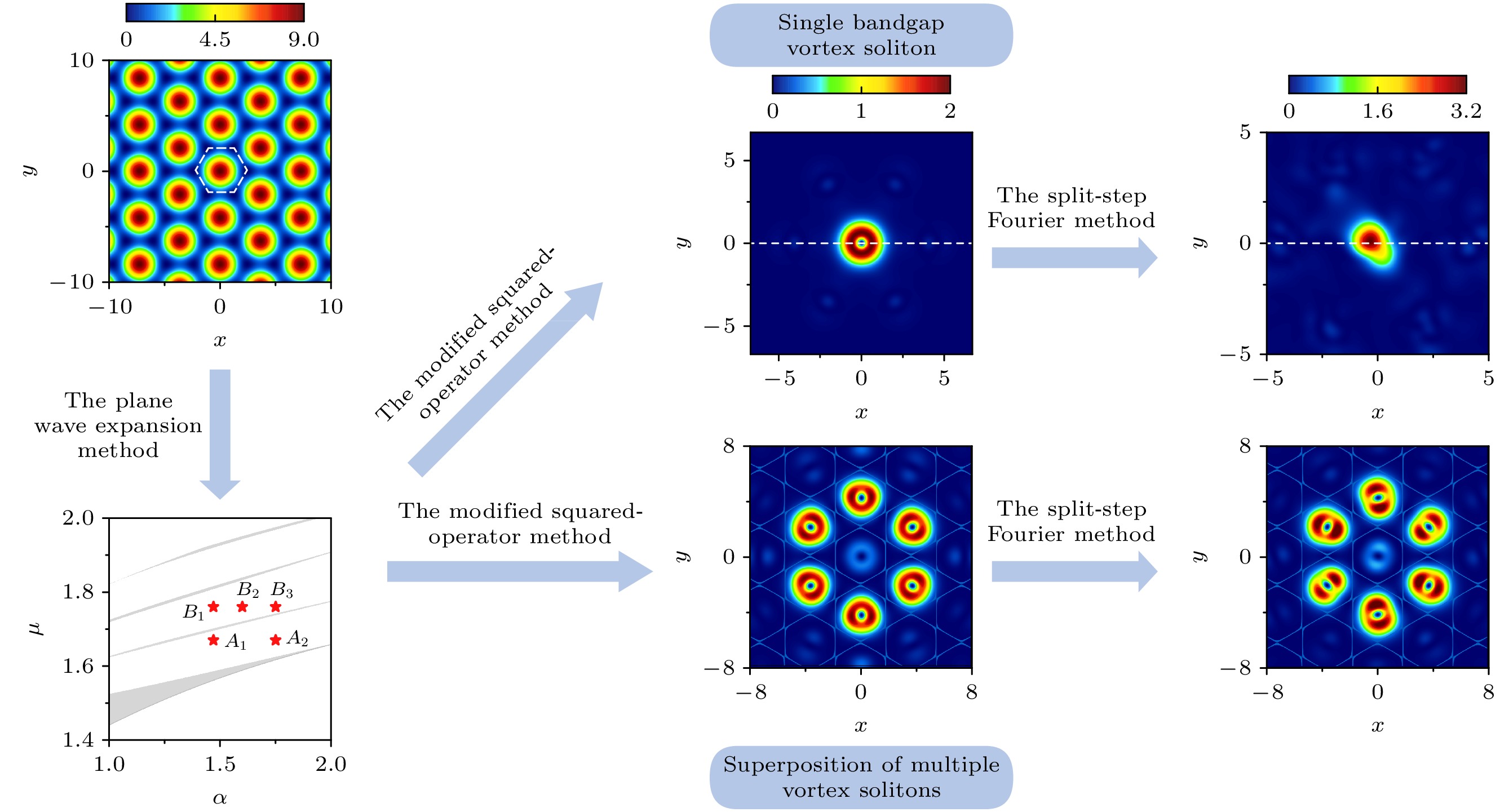
[1] 廖秋雨, 胡恒洁, 陈懋薇, 石逸, 赵元, 花春波, 徐四六, 傅其栋, 叶芳伟, 周勤 2023 物理学报 72 104202
 Google Scholar
Liao Q Y, Hu H J, Chen M W, Shi Y, Zhao Y, Hua C B, Xu S L, Fu Q D, Ye F W, Zhou Q 2023 Acta Phys. Sin. 72 104202
Google Scholar
[2] Shao Z, Wang C, Wu K, Zhang H, Chen J 2019 Nanoscale Adv. 1 4190
Google Scholar
[3] Sheng-Chyan L, Varrazza R, Siyuan Y 2006 IEEE J. Sel. Top. Quantum Electron. 12 817
Google Scholar
[4] Sang Y, Wu X, Raja S S, Wang C Y, Li H, Ding Y, Liu D, Zhou J, Ahn H, Gwo S, Shi J 2018 Adv. Opt. Mater. 6 1701368
Google Scholar
[5] Laskin N 2002 Phys. Rev. E 66 056108
Google Scholar
[6] Laskin N 2000 Phys. Rev. E 62 3135
Google Scholar
[7] Laughlin R B 1983 Phys. Rev. Lett. 50 1395
Google Scholar
[8] Wen J, Zhang Y, Xiao M 2013 Adv. Opt. Photonics 5 83
Google Scholar
[9] Rokhinson L P, Liu X, Furdyna J K 2012 Nat. Phys. 8 795
Google Scholar
[10] Olivar-Romero F, Rosas-Ortiz O 2016 J. Phys. Conf. Ser. 698 012025
Google Scholar
[11] Stickler B A 2013 Phys. Rev. E 88 012120
Google Scholar
[12] Longhi S 2015 Opt. Lett. 40 1117
Google Scholar
[13] Zhang Y, Zhong H, Belić M R, Ahmed N, Zhang Y, Xiao M 2016 Sci. Rep. 6 23645
Google Scholar
[14] Zhang A X, Zhang Y, Jiang Y F, Yu Z F, Cai L X, Xue J K 2020 Chin. Phys. B 29 010307
Google Scholar
[15] Zhang Y, Zhong H, Belić M R, Zhu Y, Zhong W, Zhang Y, Christodoulides D N, Xiao M 2016 Laser Photonics Rev. 10 526
Google Scholar
[16] Liu S, Zhang Y, Malomed B A, Karimi E 2023 Nat. Commun. 14 222
Google Scholar
[17] Zhang L, Li C, Zhong H, Xu C, Lei D, Li Y, Fan D 2016 Opt. Express 24 14406
Google Scholar
[18] He S, Zhou K, Malomed B A, Mihalache D, Zhang L, Tu J, Wu Y, Zhao J, Peng X, He Y, Zhou X, Deng D 2021 J. Opt. Soc. Am. B 38 3230
Google Scholar
[19] Zhang L, Zhang X, Wu H, Li C, Pierangeli D, Gao Y, Fan D 2019 Opt. Express 27 27936
Google Scholar
[20] Huang C, Dong L 2016 Opt. Lett. 41 5636
Google Scholar
[21] Zhu Y, Yang J, Li J, Hu L, Zhou Q 2022 Nonlinear Dyn. 109 1047
Google Scholar
[22] Huang C, Dong L 2019 Opt. Lett. 44 5438
Google Scholar
[23] Wu Z, Cao S, Che W, Yang F, Zhu X, He Y 2020 Results Phys. 19 103381
Google Scholar
[24] Wang J, Wu Q, Du C, Yang L, Xue P, Fan L 2023 Phys. Lett. A 471 128794
Google Scholar
[25] 温嘉美, 薄文博, 温学坤, 戴朝卿 2023 物理学报 72 100502
Google Scholar
Wen J M, Bo W B, Wen X K and Dai C Q 2023 Acta Phys. Sin. 72 100502
Google Scholar
[26] Zeng L, Zeng J 2020 Commun. Phys. 3 26
Google Scholar
[27] Paredes A, Salgueiro J R, Michinel H 2022 Physica D 437 133340
Google Scholar
[28] Yao X, Liu X 2018 Opt. Lett. 43 5749
Google Scholar
[29] Wang J, Jin Y, Gong X, Yang L, Chen J, Xue P 2022 Opt. Express 30 8199
Google Scholar
[30] Yao G, Li Y, Chen R P 2022 Photonics 9 249
Google Scholar
[31] Dong L, Huang C 2019 Nonlinear Dyn. 98 1019
Google Scholar
[32] Liu X, Zeng J 2024 Front. Phys. 19 42201
Google Scholar
[33] Malomed B A 2021 Photonics 8 353
Google Scholar
[34] Liu X, Malomed B A, Zeng J 2022 Adv. Theory Simul. 5 2100482
Google Scholar
[35] Zeng L, Zeng J 2019 Nonlinear Dyn. 98 985
Google Scholar
[36] Li L, Li H G, Ruan W, Leng F C, Luo X B 2020 J. Opt. Soc. Am. B 37 488
Google Scholar
[37] Liu X, Zeng J 2023 Photonics Res. 11 196
Google Scholar
[38] Peleg O, Bartal G, Freedman B, Manela O, Segev M, Christodoulides D N 2007 Phys. Rev. Lett. 98 103901
Google Scholar
[39] 黄学勤, 陈子亭 2015 物理学报 64 184208
Google Scholar
Huang X Q, Chan C T 2015 Acta Phys. Sin. 64 184208
Google Scholar
[40] Bahat-Treidel O, Peleg O, Grobman M, Shapira N, Segev M, Pereg-Barnea T 2010 Phys. Rev. Lett. 104 063901
Google Scholar
[41] Ablowitz M J, Nixon S D, Zhu Y 2009 Phys. Rev. A 79 053830
Google Scholar
[42] Yang J 2010 Mathematical Modeling and Computation (Philadelphia: the Society for Industrial and Applied Mathematics) pp271–275, 377–380
[43] Huang X, Tan W, Jiang T, Nan S, Bai Y, Fu X 2023 Opt. Commun. 527 128970
Google Scholar
-
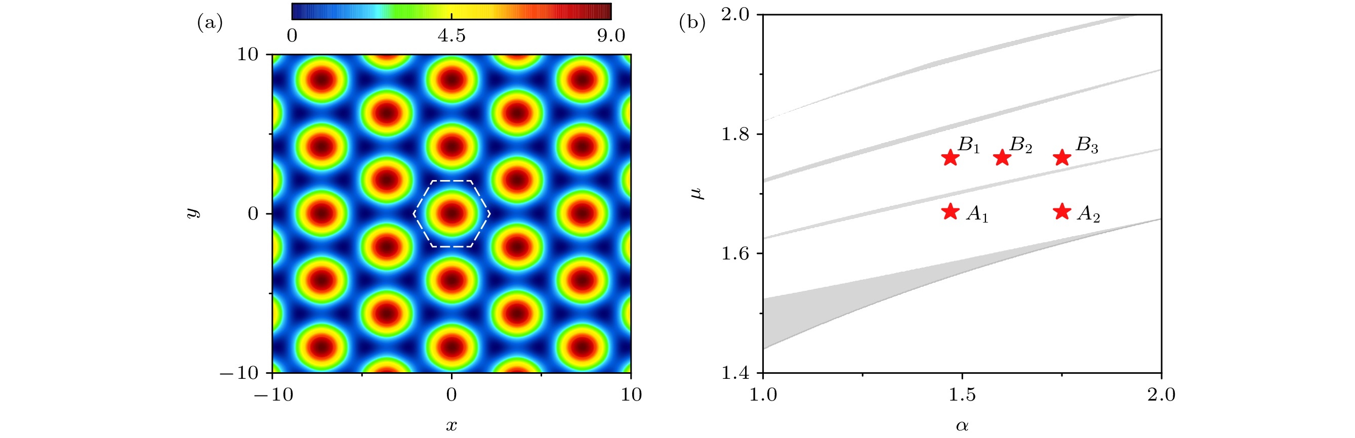
图 1 (a)蜂窝晶格结构; (b)蜂窝晶格所对应的能带结构. 其中势深 $ {V_0} = 1 $, $ {A_1}(1.47, {\text{ }}1.65) $, $ {A_2}(1.75, {\text{ }}1.65) $, $ {B_1}(1.47, {\text{ }}1.76) $, $ {B_2}(1.6, {\text{ }}1.76) $, $ {B_3}(1.75, {\text{ }}1.76) $
Figure 1. (a) Honeycomb lattice shape; (b) the corresponding band-gap structure. The potential depth is $ {V_0} = 1 $, $ {A_1}(1.47, {\text{ }}1.65) $, $ {A_2}(1.75, {\text{ }}1.65) $, $ {B_1}(1.47, {\text{ }}1.76) $, $ {B_2}(1.6, {\text{ }}1.76) $ , $ {B_3}(1.75, {\text{ }}1.76) $.
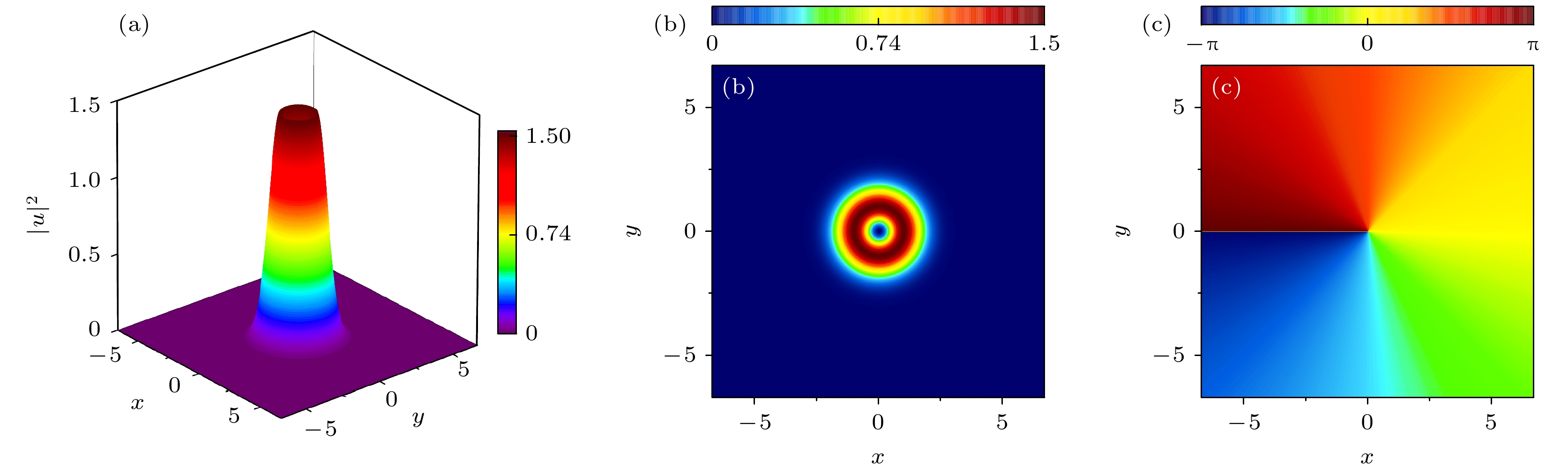
图 2 初始输入涡旋光束的强度三维分布图(a)和俯视图(b), 以及相位分布图(c). 这里取参数$ A = 2 $, $ {r_0} = \sqrt 2 $, $ l = 1 $
Figure 2. The 3D intensity distribution of initial input vortex beam (a) and corresponding top view (b), and phase distribution (c). The parameters are $ A = 2 $, $ {r_0} = \sqrt 2 $, $ l = 1 $
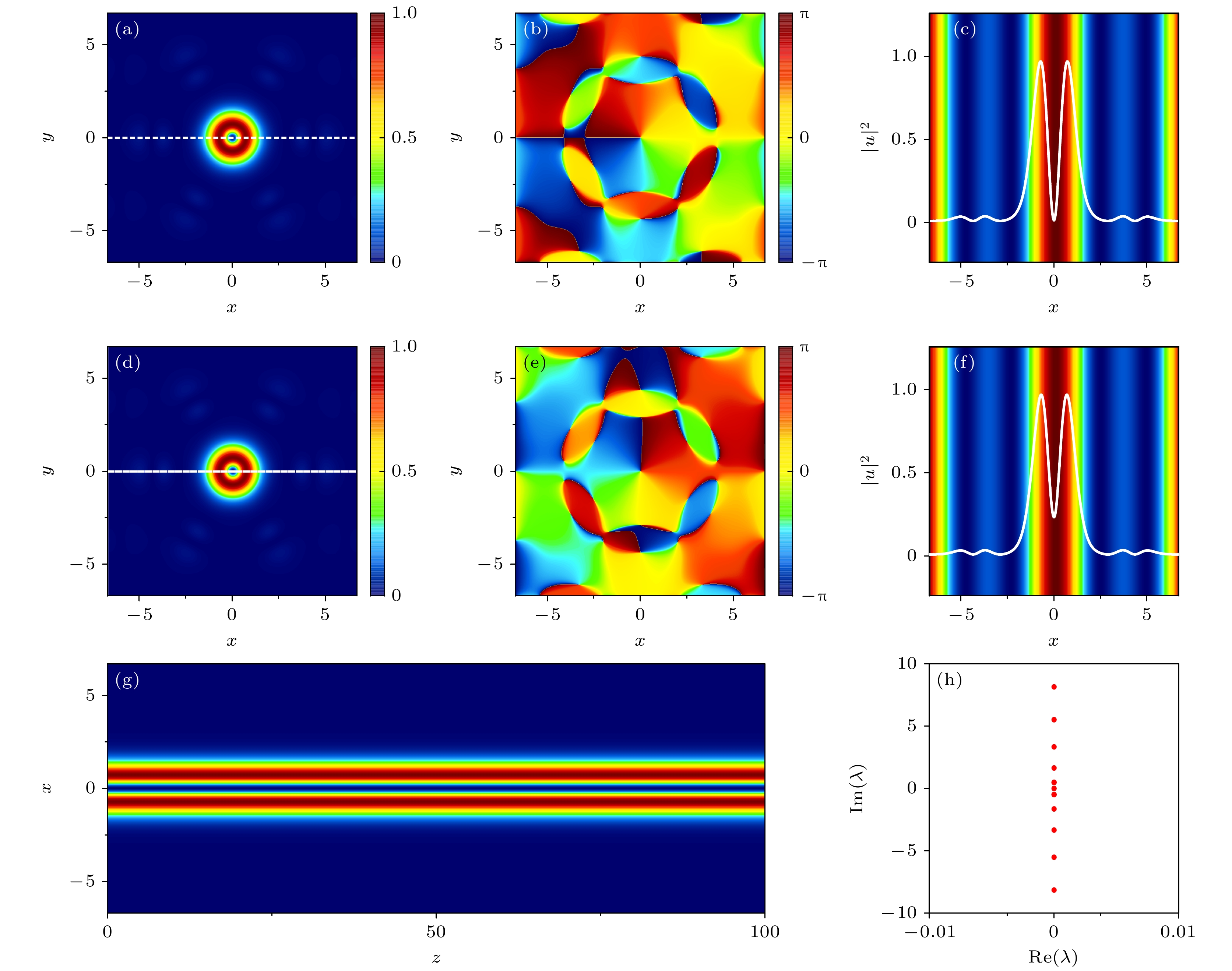
图 3 当$ \alpha = 1.75 $时, 第一带隙中带隙涡旋孤子解及稳定性分析 (a)—(c)带隙涡旋孤子解; (d)—(f)在$ z = 100 $处输出带隙涡旋孤子; (g) 带隙涡旋孤子在蜂窝晶格x方向剖面中的传输演化图; (h) 线性稳定谱图. 其他参数同图2
Figure 3. Gap vortex solitons and their stability in the first gap when $ \alpha = 1.75 $: (a)–(c) The gap vortex soliton solution; (d)–(f) the output gap vortex solitons at $ z = 100 $; (g) the transmission evolution of gap vortex soliton in the x-direction of honeycomb lattice; (h) the corresponding stable spectrum. The other parameters are the same as in Figure 2.
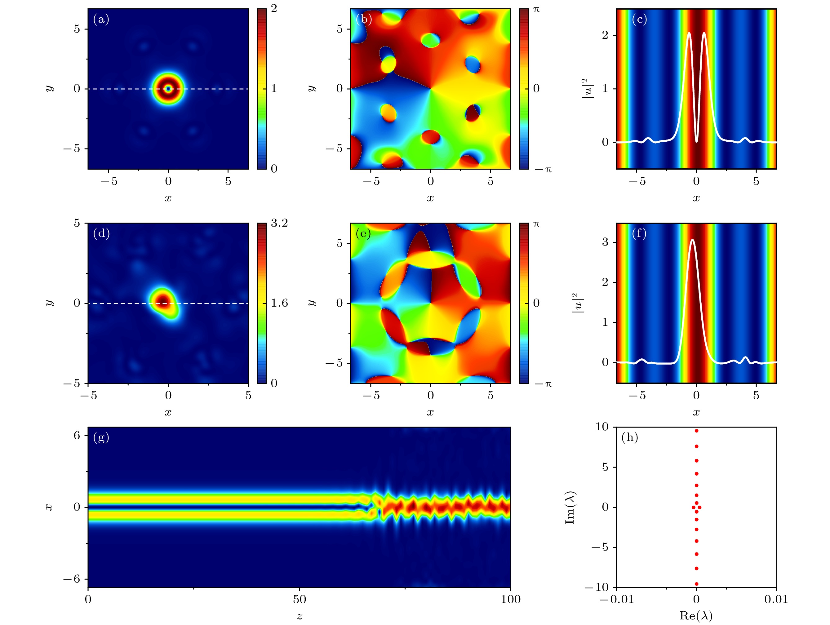
图 4 当$ \alpha = 1.47 $时, 第一带隙中带隙涡旋孤子及稳定性分析 (a)—(c)带隙涡旋孤子解; (d)—(f)在$ z = 100 $处输出带隙涡旋孤子; (g) 带隙涡旋孤子传输动力学演化; (h) 线性稳定值谱图. 其他参数同图2
Figure 4. Gap vortex solitons and their stability in the first gap when $ \alpha = 1.47 $: (a)–(c) The gap vortex soliton solution; (d)–(f) the output gap vortex solitons at $ z = 100 $; (g) the transmission evolution of gap vortex soliton in the x-direction of honeycomb lattice; (h) the corresponding stable spectrum. The other parameters are the same as in Figure 2.
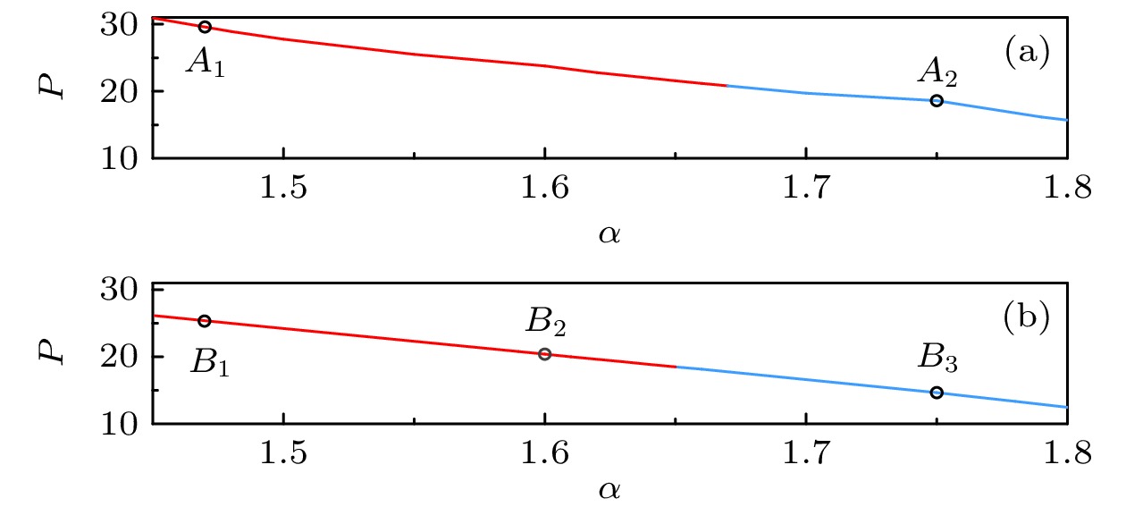
图 5 带隙涡旋孤子功率$ P $与$ {\mathrm{L}}\acute{{\mathrm{e}}}{\mathrm{v}}{\mathrm{y}} $指数$ \alpha $关系图 (a) 第一带隙的功率谱图; (b) 第二带隙的功率谱
Figure 5. Power $ P $ of gap vortex soliton versus $ {\mathrm{L}}\acute{{\mathrm{e}}}{\mathrm{v}}{\mathrm{y}} $ index $ \alpha $: (a) The power spectrum of first band gap; (b) the power spectrum of second band gap.
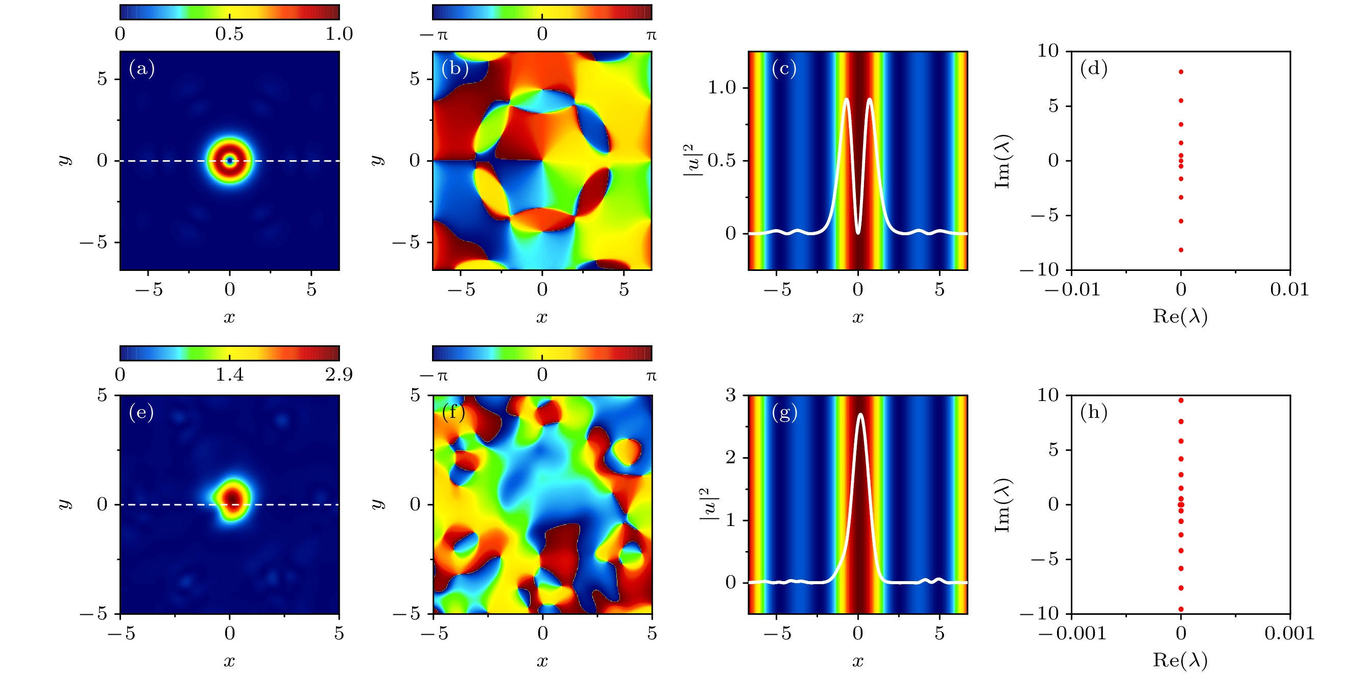
图 6 第二带隙中带隙涡旋孤子及稳定性分析 (a)—(c) 当$ \alpha = 1.75 $时, 输出带隙涡旋孤子图像; (d)—(f) 当$ \alpha = 1.47 $时, 输出带隙涡旋孤子图像; 其他参数同图2
Figure 6. Gap vortex solitons and their stability in the second gap: (a)–(c) When $ \alpha = 1.75 $, the output of vortex soliton; (d)–(f) when $ \alpha = 1.47 $, the output of vortex soliton. The other parameters are the same as that in Figure 2.
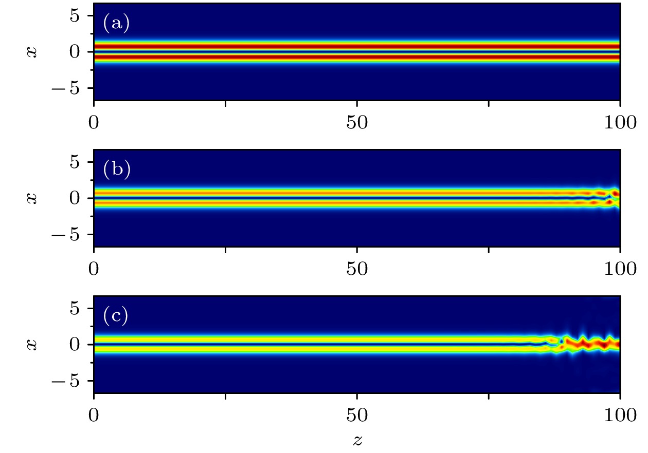
图 7 第二带隙中, 不同$ {\mathrm{L}}\acute{{\mathrm{e}}}{\mathrm{v}}{\mathrm{y}} $指数$ \alpha $下, 带隙涡旋孤子传输动力学演化图像 (a) $ \alpha = 1.75 $; (b) $ \alpha = 1.6 $; (c) $ \alpha = 1.47 $; 其他参数同图2
Figure 7. Transmission evolution of gap vortex solitons in the second gap with different $ {\mathrm{L}}\acute{{\mathrm{e}}}{\mathrm{v}}{\mathrm{y}} $ indexs: (a) $ \alpha = 1.75 $; (b) $ \alpha = 1.6 $; (c) $ \alpha = 1.47 $. The other parameters are the same as that in Figure 2.
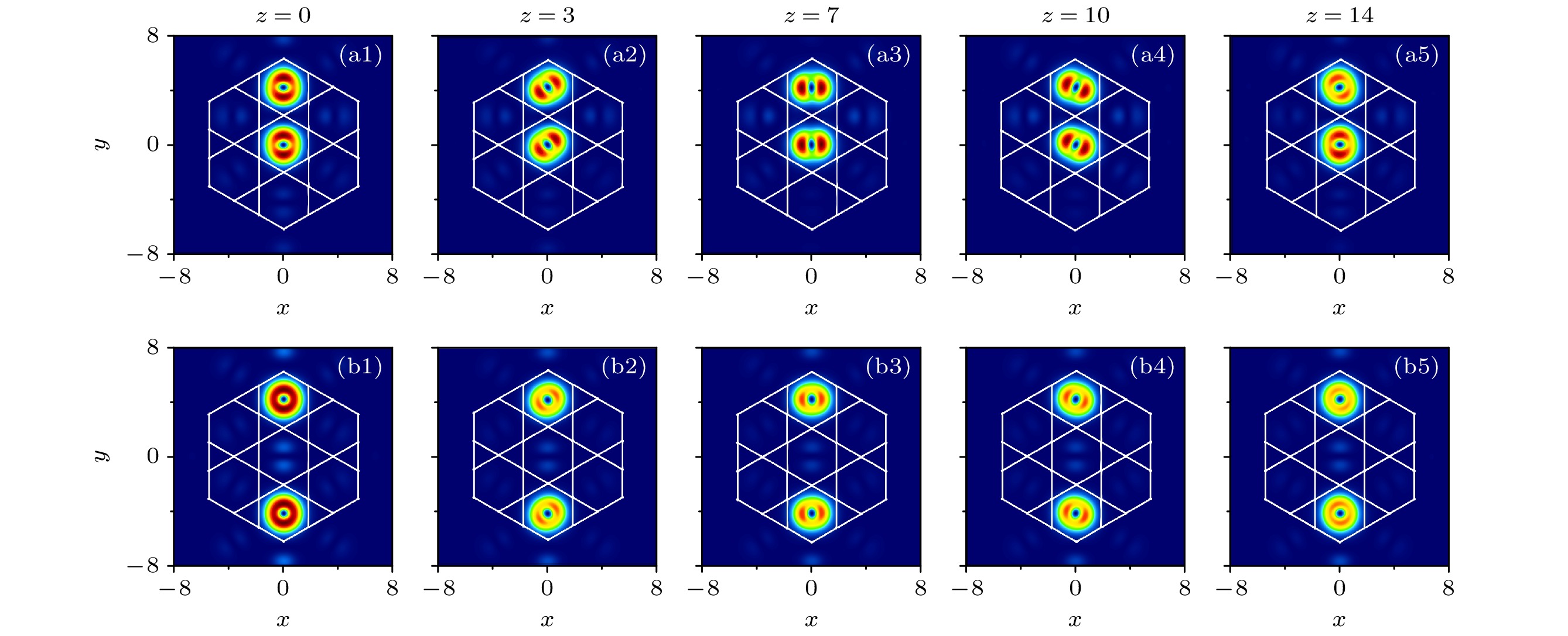
图 8 当$ \alpha = 1.8 $ 时, 在第一带隙中, 相邻((a1)—(a5))与不相邻((b1)—(b5))晶格处两个同相位带隙涡旋孤子的传输特性. 其他参数同图2
Figure 8. When $ \alpha = 1.8 $, the transmission characteristics of two gap vortex soliton with in-phase at adjacent lattices ((a1)–(a5)) and nonadjacent lattices ((b1)–(b5)) in the first gap. The other parameters are the same as that in Figure 2.
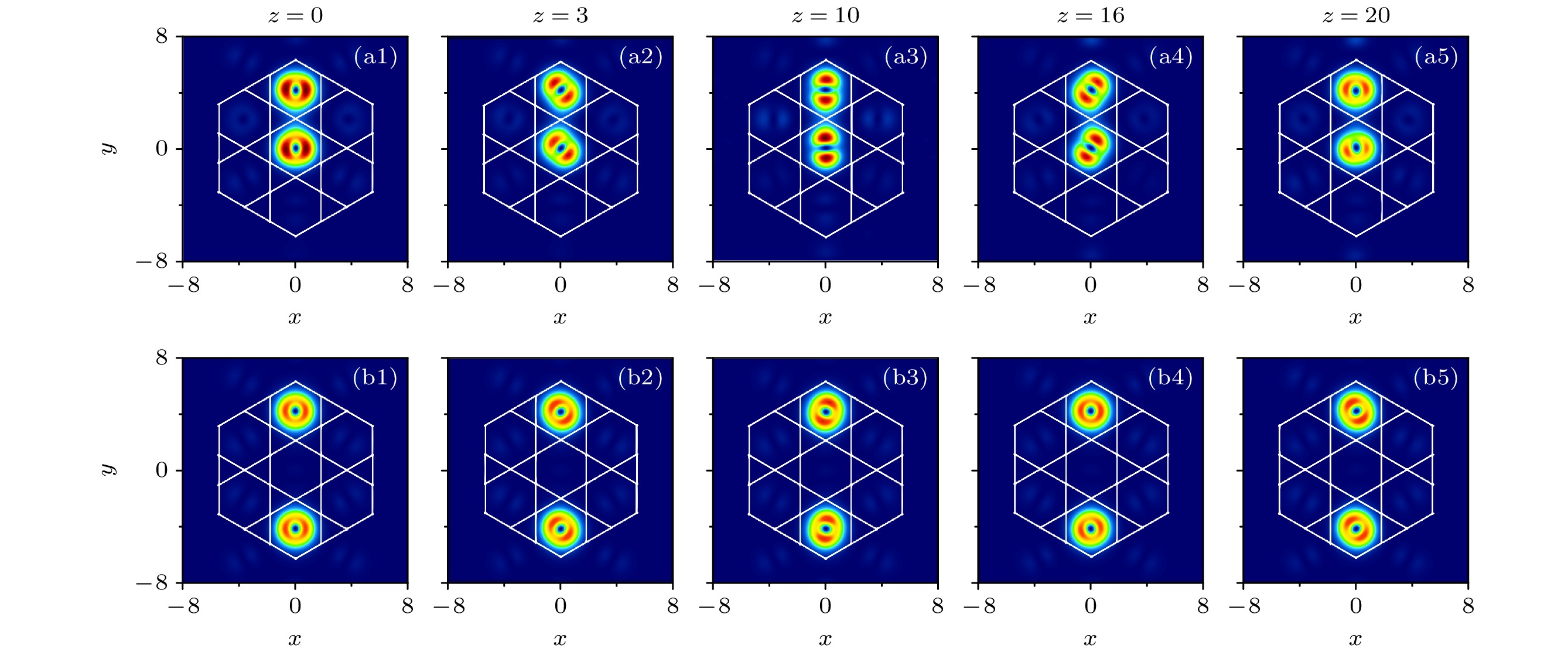
图 9 当$ \alpha = 1.8 $ 时, 在第一带隙中, 相邻((a1)—(a5))与不相邻((b1)—(b5))晶格处两个相位相反的带隙涡旋孤子传输特性. 其他参数同图2
Figure 9. When $ \alpha = 1.8 $, the transmission characteristics of two gap vortex soliton with out of phase at adjacent lattices ((a1)–(a5)) and nonadjacent lattices ((b1)–(b5)) in the first gap. The other parameters are the same as that in Figure 2.
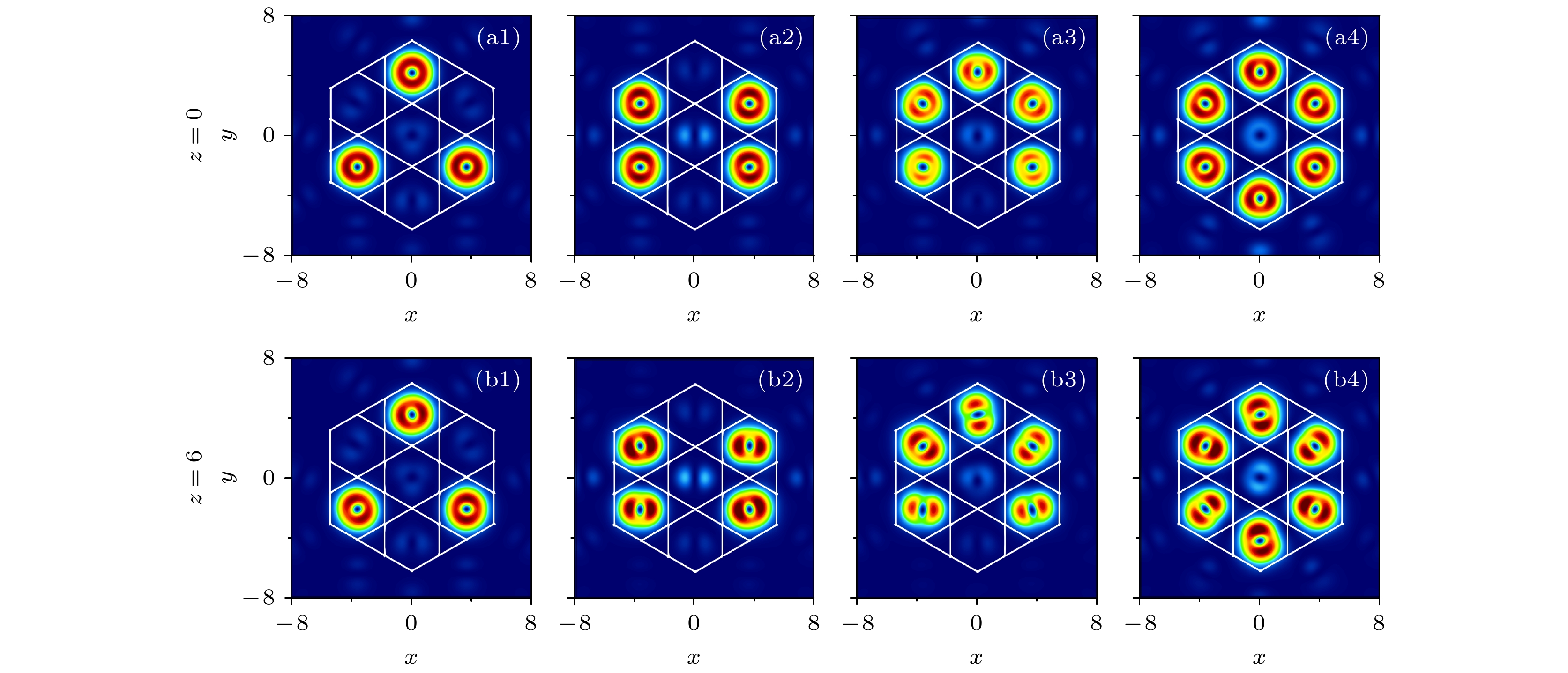
图 10 多个带隙涡旋孤子的输入($ z = 0 $)和输出($ z = 6 $)的光强分布图 (a1), (b1)三个带隙涡旋孤子; (a2), (b2) 四个带隙涡旋孤子; (a3), (b3) 五个带隙涡旋孤子; (a4), (b4) 六个带隙涡旋孤子; 其他参数同图2
Figure 10. Intensity distributions of multiple gap vortex solitons at z = 0 and z = 6: (a1), (b1) Three gap vortex solitons; (a2), (b2) four gap vortex solitons; (a3), (b3) five gap vortex solitons; (a4), (b4) six gap vortex solitons. The other parameters are the same as that in Figure 2.
-
[1] 廖秋雨, 胡恒洁, 陈懋薇, 石逸, 赵元, 花春波, 徐四六, 傅其栋, 叶芳伟, 周勤 2023 物理学报 72 104202
Google Scholar
Liao Q Y, Hu H J, Chen M W, Shi Y, Zhao Y, Hua C B, Xu S L, Fu Q D, Ye F W, Zhou Q 2023 Acta Phys. Sin. 72 104202
Google Scholar
[2] Shao Z, Wang C, Wu K, Zhang H, Chen J 2019 Nanoscale Adv. 1 4190
Google Scholar
[3] Sheng-Chyan L, Varrazza R, Siyuan Y 2006 IEEE J. Sel. Top. Quantum Electron. 12 817
Google Scholar
[4] Sang Y, Wu X, Raja S S, Wang C Y, Li H, Ding Y, Liu D, Zhou J, Ahn H, Gwo S, Shi J 2018 Adv. Opt. Mater. 6 1701368
Google Scholar
[5] Laskin N 2002 Phys. Rev. E 66 056108
Google Scholar
[6] Laskin N 2000 Phys. Rev. E 62 3135
Google Scholar
[7] Laughlin R B 1983 Phys. Rev. Lett. 50 1395
Google Scholar
[8] Wen J, Zhang Y, Xiao M 2013 Adv. Opt. Photonics 5 83
Google Scholar
[9] Rokhinson L P, Liu X, Furdyna J K 2012 Nat. Phys. 8 795
Google Scholar
[10] Olivar-Romero F, Rosas-Ortiz O 2016 J. Phys. Conf. Ser. 698 012025
Google Scholar
[11] Stickler B A 2013 Phys. Rev. E 88 012120
Google Scholar
[12] Longhi S 2015 Opt. Lett. 40 1117
Google Scholar
[13] Zhang Y, Zhong H, Belić M R, Ahmed N, Zhang Y, Xiao M 2016 Sci. Rep. 6 23645
Google Scholar
[14] Zhang A X, Zhang Y, Jiang Y F, Yu Z F, Cai L X, Xue J K 2020 Chin. Phys. B 29 010307
Google Scholar
[15] Zhang Y, Zhong H, Belić M R, Zhu Y, Zhong W, Zhang Y, Christodoulides D N, Xiao M 2016 Laser Photonics Rev. 10 526
Google Scholar
[16] Liu S, Zhang Y, Malomed B A, Karimi E 2023 Nat. Commun. 14 222
Google Scholar
[17] Zhang L, Li C, Zhong H, Xu C, Lei D, Li Y, Fan D 2016 Opt. Express 24 14406
Google Scholar
[18] He S, Zhou K, Malomed B A, Mihalache D, Zhang L, Tu J, Wu Y, Zhao J, Peng X, He Y, Zhou X, Deng D 2021 J. Opt. Soc. Am. B 38 3230
Google Scholar
[19] Zhang L, Zhang X, Wu H, Li C, Pierangeli D, Gao Y, Fan D 2019 Opt. Express 27 27936
Google Scholar
[20] Huang C, Dong L 2016 Opt. Lett. 41 5636
Google Scholar
[21] Zhu Y, Yang J, Li J, Hu L, Zhou Q 2022 Nonlinear Dyn. 109 1047
Google Scholar
[22] Huang C, Dong L 2019 Opt. Lett. 44 5438
Google Scholar
[23] Wu Z, Cao S, Che W, Yang F, Zhu X, He Y 2020 Results Phys. 19 103381
Google Scholar
[24] Wang J, Wu Q, Du C, Yang L, Xue P, Fan L 2023 Phys. Lett. A 471 128794
Google Scholar
[25] 温嘉美, 薄文博, 温学坤, 戴朝卿 2023 物理学报 72 100502
Google Scholar
Wen J M, Bo W B, Wen X K and Dai C Q 2023 Acta Phys. Sin. 72 100502
Google Scholar
[26] Zeng L, Zeng J 2020 Commun. Phys. 3 26
Google Scholar
[27] Paredes A, Salgueiro J R, Michinel H 2022 Physica D 437 133340
Google Scholar
[28] Yao X, Liu X 2018 Opt. Lett. 43 5749
Google Scholar
[29] Wang J, Jin Y, Gong X, Yang L, Chen J, Xue P 2022 Opt. Express 30 8199
Google Scholar
[30] Yao G, Li Y, Chen R P 2022 Photonics 9 249
Google Scholar
[31] Dong L, Huang C 2019 Nonlinear Dyn. 98 1019
Google Scholar
[32] Liu X, Zeng J 2024 Front. Phys. 19 42201
Google Scholar
[33] Malomed B A 2021 Photonics 8 353
Google Scholar
[34] Liu X, Malomed B A, Zeng J 2022 Adv. Theory Simul. 5 2100482
Google Scholar
[35] Zeng L, Zeng J 2019 Nonlinear Dyn. 98 985
Google Scholar
[36] Li L, Li H G, Ruan W, Leng F C, Luo X B 2020 J. Opt. Soc. Am. B 37 488
Google Scholar
[37] Liu X, Zeng J 2023 Photonics Res. 11 196
Google Scholar
[38] Peleg O, Bartal G, Freedman B, Manela O, Segev M, Christodoulides D N 2007 Phys. Rev. Lett. 98 103901
Google Scholar
[39] 黄学勤, 陈子亭 2015 物理学报 64 184208
Google Scholar
Huang X Q, Chan C T 2015 Acta Phys. Sin. 64 184208
Google Scholar
[40] Bahat-Treidel O, Peleg O, Grobman M, Shapira N, Segev M, Pereg-Barnea T 2010 Phys. Rev. Lett. 104 063901
Google Scholar
[41] Ablowitz M J, Nixon S D, Zhu Y 2009 Phys. Rev. A 79 053830
Google Scholar
[42] Yang J 2010 Mathematical Modeling and Computation (Philadelphia: the Society for Industrial and Applied Mathematics) pp271–275, 377–380
[43] Huang X, Tan W, Jiang T, Nan S, Bai Y, Fu X 2023 Opt. Commun. 527 128970
Google Scholar


 DownLoad:
Catalog
Metrics
- Abstract views: 4254
- PDF Downloads: 127
- Cited By: 0
