Complex exponential reconstruction algorithm accelerated by cascadic multigrid method

Zhao Wang; Dong Li-Zhi; Yang Ping; Wang Shuai; Xu Bing

doi:10.7498/aps.68.20182137

Abstract

Authors and contacts

FullText HTML

1. 引　言
2. 复指数波前复原算法
3. 瀑布型多重网格法
4. CMG算法波前复原性能
5. 采用CMG算法的自适应光学系统校正能力
5.1 激光大气传输补偿系统数值仿真
5.2 自适应光学系统校正效果
6. 结　论

References

Cited By

Abstract

When laser beam propagates through the turbulent atmosphere, there are branch points in wavefront, which are caused by deep turbulence or long propagation distance. Conventional least-square reconstruction algorithms cannot restore the discontinuous wavefront, which severely limits correction performance of an adaptive optics system. If the incoming wavefront contains a branch cut, there is

${\rm{2}}n{\text{π}}$ difference between the measured phase difference and the principle phase difference, which is the reason why conventional least-square reconstruction algorithms cannot reconstruct wavefront with branch points. The complex exponential reconstructor is developed to restore the discontinuous wavefront with phase difference replaced by complex exponents. However, thousands of iterations are required by the complex exponential reconstructor before converging to an acceptable solution. In order to speed up the iterative calculation, the cascadic multigrid method (CMG) is introduced in the process of wavefront reconstruction. The proposed method can be used to restore discontinuous wavefront with lower residual error similar to those reconstructed by the direct iteration. The number of float point multiplications required by the CMG method is nearly 2 orders of magnitude lower than that required by the direct iteration. The acceleration of the CMG method increases with the number of subapertures increasing. The performance of CMG method to recover continuous wavefront is also investigated and compared with conventional wavefront reconstruction algorithm based on successive over-relaxation. It is shown that the CMG method has good capability for wavefront reconstruction with high precision and low computation cost no matter whether it is applied to discontinuous or continuous wavefront. Furthermore, the CMG method is used in the adaptive optics for correcting the turbulence aberration. The direct slope wavefront reconstruction algorithm based on the assumption that the measured slope and the control voltage satisfy the linear relationship cannot restore the wavefront with branch points. As a result, the adaptive optics system with the CMG method doubles the correction quality evaluated by the Strehl ratio compared with that with the direct slope wavefront reconstruction algorithm.

Keywords:

PACS:

42.68.Wt	(Remote sensing; LIDAR and adaptive systems)
95.75.Qr	(Adaptive and segmented optics)
42.68.Bz	(Atmospheric turbulence effects)

Authors and contacts

1.
Key Laboratory on Adaptive Optics, Chinese Academy of Sciences, Chengdu 610209, China
2.
Institute of Optics and Electronics, Chinese Academy of Sciences, Chengdu 610209, China
3.
University of Chinese Academy of Sciences, Beijing 100049, China

Corresponding author: Wang Shuai, wangshuai@ioe.ac.cn

Funds: Project supported by the National Natural Science Foundation of China (Grant No. 61875203), the Young Scientists Fund of the National Natural Science Foundation of China (Grant Nos. 11704382, 61805251), and the International (Regional) Cooperation and Exchange Program of the National Natural Science Foundation of China (Grant No. 1171101412).

FullText HTML

1. 引　言

激光在大气中传输时, 由于强湍流或长传输距离的影响, 会出现强闪烁效应, 此时波前中出现相位不连续点^[1,2]. 常规波前复原算法不能准确复原波前中的不连续结构, 使得自适应光学系统校正效果下降甚至失效^[3-5]. 为了解决该问题, Le等^[6]开展了复指数因子波前复原算法(complex exponential reconstructor, CER)研究, 其将相位差用复指数表示, 利用迭代计算实现了对单个相位奇点的复原, 该方法需要上万次迭代才能收敛, 实用性差. Fried^[7]和Barchers等^[8]将CER算法中迭代计算简化为降采样、最小二乘求解、数据重构三个过程, 实现了对CER算法的加速. 但是该方法要求子孔径数目满足 ${2^N} \times {2^N}$ , 子孔径数目不满足要求时, 需要对子孔径进行扩充, 使得波前复原结果存在较大误差. 同时, 通光口径不是正方形时, 由于引入过多的权值为零数据点, 波前复原结果将存在较大残差. 此外, Aubailly 和Vorontsov^[9]以及Yazdani 和Fallah^[10]将相位恢复算法用于相位奇点复原, 此方法需要测量微透镜后不同位置的光强数据, 利用光传输原理复原波前. 其光强测量系统复杂, 波前复原算法计算量大, 难以应用于自适应光学系统.

为了解决复指数波前复原算法计算量大的问题, 本文提出了基于瀑布型多重网格(cascadic multigrid method, CMG)加速的复指数波前复原算法，该算法利用夏克-哈特曼波前传感器测量相位差给出不同网格层上光场间的关系, 在最粗网格上计算满足收敛条件的解, 并将其插值到细网格层, 作为该层迭代计算的初值, 减少了迭代计算次数, 加速了波前复原过程. 本文利用CMG算法和直接迭代复原了不连续相位和随机连续相位，比较了两种波前复原算法的波前复原精度和算法复杂度，对比了采用CMG算法和直接斜率法的自适应光学系统对大气湍流像差的校正效果, 并给出了相应结论.

2. 复指数波前复原算法

由傅里叶光学可知第i个子孔径焦平面上光场复振幅^[11]为

$\begin{split} u\left( {{x_f},{y_f}} \right) =& \frac{{\exp \left[ {{\rm{i}}\frac{k}{{2f}}\left( {x_f^2 + y_f^2} \right)} \right]}}{{{\rm{i}}\lambda f}} \centerdot\iint_{ - \infty }^\infty u\left( {{x_0},{y_0}} \right)\\ &\times\exp \left( { - \frac{{2{\text{π}}}}{{\lambda f}}\left( {{x_0}{x_f} + {y_0}{y_f}} \right)} \right){\rm{d}}{x_0}{\rm{d}}{y_0}, \end{split}$

(1)

式中 $u\left( {{x_0},{y_0}} \right)$ 为入射光场复振幅, $\lambda$ 为激光波长, $f$ 为微透镜焦距, $k = 2{\text{π}} /\lambda$ .

焦平面上光强分布为

$I\left( {{x_f},{y_f}} \right) = {\left| {u\left( {{x_f},{y_f}} \right)} \right|^2} = \frac{1}{{{{\left( {\lambda f} \right)}^2}}}{\left| {U\left( {u,v} \right)} \right|^2},$

(2)

式中

$U\!\left( {u,v} \right) \!=\!\!\! {\displaystyle\iint_{ - \infty }^\infty \!\!{u\left( {{x_0},{y_0}} \right)\exp \left(\!{ - 2{\text{π}}\left( {{x_0}u \!+\! {y_0}v} \right)} \right){\rm{d}}{x_0}{\rm{d}}{y_0}} }$ , 表示入射光场的傅里叶变换, $u=\dfrac{{{x_f}}}{{\lambda f}}$ , $v=\dfrac{{{y_f}}}{{\lambda f}}$ 表示x, y方向的空间频率.

子孔径聚焦光斑x方向质心位置为

$\begin{split}{x_{\rm{c}}}&= \frac{{{\displaystyle\iint_{ - \infty }^\infty {{x_f}I\left( {{x_f},{y_f}} \right){\rm{d}}{x_f}{\rm{d}}{y_f}} } }}{{{\displaystyle\iint_{ - \infty }^\infty {I\left( {{x_f},{y_f}} \right){\rm{d}}{x_f}{\rm{d}}{y_f}} } }} \\&= \frac{{\lambda f{\displaystyle\iint_{ - \infty }^\infty {uU\left( {u,v} \right){U^ * }\left( {u,v} \right){\rm{d}}u{\rm{d}}v} } }}{{{\displaystyle\iint_{ - \infty }^\infty {{{\left| {U\left( {u,v} \right)} \right|}^2}{\rm{d}}u{\rm{d}}v} } }}.\end{split}$

(3)

由傅里叶变换微分性质和卷积定理可得:

$\begin{split}&{\rm{i}}2{\text{π}}uU\left( {u,v} \right){U^ * }\left( {u,v} \right)={\iint_{ - \infty }^\infty {C\left( {x,y} \right)} }\\ &\times\exp \left( { - {\rm{i}}2{\text{π}}\left( {xu + yv} \right)} \right){\rm{d}}x{\rm{d}}y,\end{split}$

(4)

其中

$\begin{split} C\left( {x,y} \right) &= \frac{{\partial u\left( {x,y} \right)}}{{\partial x}} \otimes {u^ * }\left( { - x, - y} \right) \\ &= {\iint_{ - \infty }^\infty {\frac{{\partial u\left( {x',y'} \right)}}{{\partial x'}}} } {u^ * }\left( {x' - x,{\rm{y}}' - y} \right){\rm{d}}x'{\rm{dy}}'. \end{split}$

(5)

利用(4)式可得

$\begin{split} {\displaystyle\iint_{ - \infty }^\infty {{\rm{i}}2{\text{π}}uU\left( {u,v} \right){U^ * }\left( {u,v} \right){\rm{d}}u{\rm{d}}v} } & ={\displaystyle\iint_{ - \infty }^\infty {\left( {{\displaystyle\iint_{ - \infty }^\infty {C\left( {x,y} \right)} } \exp \left( { - {\rm{i}}2{\text{π}}\left( {xu + yv} \right)} \right){\rm{d}}x{\rm{d}}y} \right){\rm{d}}u{\rm{d}}v} } \\ & ={\displaystyle\iint_{ - \infty }^\infty {C\left( {x,y} \right)} } \left( {{\displaystyle\iint_{ - \infty }^\infty {\exp\left( { - {\rm{i}}2{\text{π}}\left( {xu + yv} \right)} \right){\rm{d}}u{\rm{d}}v} } } \right){\rm{d}}x{\rm{d}}y \\ & ={\displaystyle\iint_{ - \infty }^\infty {\left( {{\displaystyle\iint_{ - \infty }^\infty {\frac{{\partial u\left( {x',y'} \right)}}{{\partial x'}}} } {u^ * }\left( {x' - x,y' - y} \right){\rm{d}}x'{\rm{d}}y'} \right)} } \delta \left( x \right)\delta \left( y \right){\rm{d}}x{\rm{d}}y \\ & ={\displaystyle\iint_{ - \infty }^\infty {\frac{{\partial u\left( {x',y'} \right)}}{{\partial x'}}} } {u^ * }\left( {x',y'} \right){\rm{d}}x'{\rm{d}}y'. \end{split}$

(6)

将(6)式代入(3)式可得x方向质心位置为:

${x_{\rm{c}}} = {\rm Re} \left[ {\frac{{\lambda f{\displaystyle\iint_{ - \infty }^\infty {\frac{{\partial u\left( {x,y} \right)}}{{\partial x}}} } {u^ * }\left( {x,y} \right){\rm{d}}x{\rm{d}}y}}{{{\rm{i}}2{\text{π}}{\displaystyle\iint_{ - \infty }^\infty {u\left( {x,y} \right){u^ * }\left( {x,y} \right){\rm{d}}x{\rm{d}}y} } }}} \right].$

(7)

同理, 子孔径聚焦光斑y方向质心位置为:

${y_{\rm{c}}} = {\rm Re} \left[ {\frac{{\lambda f{\displaystyle\iint_{ - \infty }^\infty {\frac{{\partial u\left( {x,y} \right)}}{{\partial y}}} } {u^ * }\left( {x,y} \right){\rm{d}}x{\rm{d}}y}}{{{\rm{i}}2{\text{π}}{\displaystyle\iint_{ - \infty }^\infty {u\left( {x,y} \right){u^ * }\left( {x,y} \right){\rm{d}}x{\rm{d}}y} } }}} \right].$

(8)

入射光波x, y方向波前斜率为:

$\begin{split} & g_{i,j}^x = \frac{{\Delta {x_{i,j}}}}{f} = \frac{{x_{i,j}^{\rm{c}} - x_{i,j}^0}}{f}, \\ & g_{i,j}^y = \frac{{\Delta {y_{i,j}}}}{f} = \frac{{y_{i,j}^{\rm{c}} - y_{i,j}^0}}{f}, \end{split}$

(9)

式中, $x_{i,j}^{\rm{c}}$ , $y_{i,j}^{\rm{c}}$ 表示第(i, j)个子孔径聚焦光斑质心位置, $x_{i,j}^0$ 和 $y_{i,j}^0$ 表示标定质心位置, f为子孔径焦距.

包含相位奇点的波前^[1]中, 枝切线(branch cut)两侧存在 $2n{\text{π}}$ 跳变. 假设某个子孔径中测量相位 $\varphi \left( x \right)$ 存在枝切线, 波前被枝切线分割成两部分, 即

$\varphi \left( x \right){\rm{ = }}\left\{ \begin{array}{l} {\varphi _t}\left( x \right)\;\;\;\;\;\;\;\;\;\;\;\;\;\;x \in {S_1} \\ {\varphi _t}\left( x \right) + 2n{\text{π}}\;\;\;\;x \in {S_2} \end{array} \right.,$

(10)

其中, ${\varphi _t}\left( x \right)$ 为不包含 $2n{\text{π}}$ 跳变的连续相位, ${S_1}$ 和 ${S_2}$ 表示被枝切线分割的两部分. 依据复指数性质有 ${{\rm{e}}^{{\rm{i}}\varphi \left( x \right)}}{\rm{ = }}{{\rm{e}}^{{\rm{i}}{\varphi _t}\left( x \right)}}$ , 由(7)式—(9)式可知, 夏克-哈特曼波前传感器不能探测波前中的 $2n{\text{π}}$ 相位跳变.

Hudgin模型^[12]中, 重建相位点在栅格点上, 测量数据是栅格点间的相位差, 如图1所示, 红色实心点表示重建相位点, 箭头表示测量相位差. 子孔径大小为d时, 第(i, j)个子孔径x, y方向测量相位差为:

$图 1 测量相位差和重建相位点的关系\r\nFig. 1. The relationship between phase differences and phase.$

图 1 测量相位差和重建相位点的关系

Fig. 1. The relationship between phase differences and phase.

下载: 全尺寸图片幻灯片

$\begin{split} & \Delta \varphi _{i,j}^x = g_{i,j}^x \times d = {\varphi _{i,j + 1}} - {\varphi _{i,j}}, \\ & \Delta \varphi _{i,j}^y = g_{i,j}^y \times d = {\varphi _{i + 1,j}} - {\varphi _{i,j}}, \end{split}$

(11)

式中, $\Delta \varphi _{i,j}^x$ , $\Delta \varphi _{i,j}^y$ 表示x, y方向测量相位差, ${\varphi _{i,j}}$ 表示重建相位点数据. 波前中不存在枝切线时, 测量相位差为相邻真实相位点的差值. 当波前中存在枝切线时, $2n{\text{π}}$ 相位跳变对斜率测量没有影响, 测量相位差为真实相位差值对 $2{\text{π}}$ 取模. 根据(11)式, 测量相位差和真实相位的关系可以表示成矩阵形式, 即

$\Delta {{{\varphi}} _{{\rm{HS}}}}{\rm{ = }}\left\{ {\begin{array}{*{20}{c}} {{{A}}{{{\varphi}} _r}{\rm{mod 2{\text{π}} , }}}&{\;{\text{存在枝切线}}}\\ {{{A}}{{{\varphi}} _r},}&{\;{\text{不存在枝切线}}} \end{array}} \right. ,$

(12)

式中, A为 + 1, 0, –1组成的稀疏矩阵, 用于表示测量相位差和真实相位的关系. $\Delta {{{\varphi}} _{{\rm{HS}}}}$ 为向量形式表示的测量相位差, ${{{\varphi}} _r}$ 为向量形式表示的真实相位.

波前中不存在枝切线时, 可以利用迭代计算求解(12)式的方程组, 迭代计算公式^[13]为:

$\begin{split} \varphi _{i,j}^{n + 1}= \,& c_{i - 1,j}^y\left( {\varphi _{i - 1,j}^n + \Delta \varphi _{i - 1,j}^y} \right) \\ & + c_{i,{\rm{j}} - 1}^x\left( {\varphi _{i,j - 1}^n + \Delta \varphi _{i,j - 1}^x} \right) \\ & + c_{i,j}^x\left( {\varphi _{i,j + 1}^n - \Delta \varphi _{i,j}^x} \right) \\ & + c_{i,j}^y\left( {\varphi _{i + 1,j}^n - \Delta \varphi _{i,j}^y} \right), \end{split}$

(13)

其中, $\varphi _{i,j}^{n + 1}$ 表示第n + 1次迭代得到的重建相位, c为权值因子. 相位点位于重建相位内部时, c = 1/4; 相位点位于重建相位边界上非顶点位置时, 相位点周围有一个方向上的相位差不存在, 如果相位点位于重建相位左边界上, 此时 $c_{i,j - 1}^x = 0$ , $c_{i - 1,j}^y = 1/3$ , $c_{i,j}^x = 1/3$ , $c_{i,j}^y = 1/3$ , 同理可得相位点位于其他边上时的权值c; 相位点位于重建相位顶点时, 相位点周围有两个方向上的相位差不存在, 如果相位点是左上角顶点, 此时 $c_{i - 1,j}^y = 0$ , $c_{i,j - 1}^x = 0$ , $c_{i,j}^x = 1/2$ , $c_{i,j}^y = 1/2$ , 同理可得重建相位点位于其他顶点时的权值c.

存在枝切线的相位中, 测量相位差和真实相位差满足 $\Delta {\varphi _{{\rm{HS}}}}{\rm{ = }}\Delta {\varphi _r} + 2n{\text{π}}$ , $\Delta {\varphi _r}$ 表示真实相位差. 此时, (13)式不满足等式关系, 不能用其重建相位. 由复指数性质, 有 ${{\rm{e}}^{{\rm{i}}\Delta {\varphi _{{\rm{HS}}}}}} = {{\rm{e}}^{{\rm{i}}\left( {\Delta {\varphi _r} + 2n{\text{π}}} \right)}} = {{\rm{e}}^{{\rm{i}}\Delta {\varphi _r}}}$ , 测量相位差和真实相位差复指数相等. 将(13)式中相位和相位差用复指数代替, 相位和相位差间的加运算变成复指数乘运算, 有

$\begin{split} {{\rm{e}}^{{\rm{i}}\varphi _{i,j}^{n + 1}}}=& c_{i - 1,j}^y{{\rm{e}}^{{\rm{i}}\varphi _{i - 1,j}^n}}{{\rm{e}}^{{\rm{i}}\Delta \varphi _{i - 1,j}^y}} + c_{i,{\rm{j}} - 1}^x{{\rm{e}}^{{\rm{i}}\varphi _{i,j - 1}^n}}{{\rm{e}}^{{\rm{i}}\Delta \varphi _{i,{\rm{j}} - 1}^x}}\\ & + c_{i,j}^x{{\rm{e}}^{{\rm{i}}\varphi _{i,j + 1}^n}}{{\rm{e}}^{ - {\rm{i}}\Delta \varphi _{i,j}^x}} + c_{i,j}^y{{\rm{e}}^{{\rm{i}}\varphi _{i + 1,j}^n}}{{\rm{e}}^{ - {\rm{i}}\Delta \varphi _{i,j}^y}}. \end{split}$

(14)

(14)式给出了复指数波前复原算法迭代计算过程, 对(14)式所得结果取矢量辐角可得重建相位. 复指数波前复原算法更为通用的迭代计算公式为:

$\begin{split} u_{i,j}^{n + 1} =\, &{\omega _{i - 1,j}}{{\rm{e}}^{{\rm{i}}\Delta \varphi _{_{i - 1,j}}^y}}u_{i - 1,j}^n + {\omega _{i,j - 1}}{{\rm{e}}^{{\rm{i}}\Delta \varphi _{_{i,j{\rm{ - }}1}}^x}}u_{i,j{\rm{ - }}1}^n \\ &+ {\omega _{i,j}}{{\rm{e}}^{{\rm{ - i}}\Delta \varphi _{_{i,j}}^x}}u_{i,j + 1}^n + {\omega _{i,j}}{{\rm{e}}^{{\rm{ - i}}\Delta \varphi _{_{i,j}}^y}}u_{i{\rm{ - }}1,j}^n, \end{split}$

(15)

式中 $u_{i,j}^{n + 1}$ 表示第n + 1次迭代计算得到的光场, ${\omega _{i,j}}$ 表示测量相位差对应的权值大小. 本文中权值等于子孔径光斑峰值信噪比, 探测器噪声为零时, 测量相位差权值等于1. 此外, 将有效通光口径外的测量相位差权值置零, 可以实现任意通光口径的波前复原.

迭代计算终止条件为

$\left| {u_{i,j}^{n + 1} - u_{i,j}^n} \right| < \varepsilon ,$

(16)

其中, $u_{i,j}^n$ 和 $u_{i,j}^{n + 1}$ 表示第n和n + 1次迭代计算得到数据, $\varepsilon$ 表示收敛精度.

3. 瀑布型多重网格法

瀑布型多重网格法^[14](cascadic multigrid method, CMG)网格结构和计算流程如图2所示, 相邻两层网格间距满足 ${h_i} = 2{h_{i{\rm{ - }}1}}$ . 图2(b)中红色方框表示最粗网格上的迭代计算, 圆点表示细网格上的迭代计算, 箭头表示插值过程. CMG算法计算流程为: 首先在最粗网格上计算满足收敛条件的解, 将其插值到细网格, 此数据作为细网格迭代计算的初值, 重复迭代计算和插值过程直到在最细网格上得到满足收敛条件的解.

$图 2 瀑布型多重网格法示意图　(a)网格结构; (b)CMG算法计算流程\r\nFig. 2. Schematic of the CMG method: (a) Structure of network layers; (b) calculation process.$

图 2 瀑布型多重网格法示意图　(a)网格结构; (b)CMG算法计算流程

Fig. 2. Schematic of the CMG method: (a) Structure of network layers; (b) calculation process.

下载: 全尺寸图片幻灯片

利用CMG算法加速(15)式时, 夏克-哈特曼波前传感器只给出了最细网格上测量相位差, 粗网格相位差需通过细网格数据降采样得到, 降采样过程如图3所示. 图3(a)中实心点表示细网格上光场, 图3(b)中实心点表示粗网格上光场, 圆圈表示剔除的细网格光场. 粗网格上相位差复指数表示为细网格上相邻复指数相乘, 即

$图 3 CMG算法降采样过程　(a)细网格上光场; (b)粗网格上光场\r\nFig. 3. Downsampling process of the CMG method: (a) Data on the fine network; (b) data on the coarse network.$

图 3 CMG算法降采样过程　(a)细网格上光场; (b)粗网格上光场

Fig. 3. Downsampling process of the CMG method: (a) Data on the fine network; (b) data on the coarse network.

下载: 全尺寸图片幻灯片

$\begin{split} &\Delta {u_{x{\rm{c}}}} = {{\rm{e}}^{{\rm{i}}\varphi _1^x}}\centerdot {{\rm{e}}^{{\rm{i}}\varphi _2^x}} = {x_1}{x_2}\\ &\Delta {u_{y{\rm{c}}}} = {{\rm{e}}^{{\rm{i}}\varphi _1^y}}\centerdot{{\rm{e}}^{{\rm{i}}\varphi _2^y}} = {y_1}{y_2}, \end{split}$

(17)

$\begin{split} & {\omega _{x{\rm{c}}}} = \frac{1}{{1/{\omega _{x1}} + 1/{\omega _{x2}}}}\\ & {\omega _{y{\rm{c}}}} = \frac{1}{{1/{\omega _{y1}} + 1/{\omega _{y2}}}}, \end{split}$

(18)

其中, $\varphi _1^x$ , $\varphi _2^x$ , $\varphi _1^y$ , $\varphi _2^y$ 为细网格上x, y方向测量相位差, x₁, x₂, y₁, y₂为细网格上相位差复指数, ${\omega _{x1}}$ , ${\omega _{x2}}$ , ${\omega _{y1}}$ , ${\omega _{y2}}$ 为测量相位差权值. $\Delta {u_{x{\rm{c}}}}$ , $\Delta {u_{y{\rm{c}}}}$ 为粗网格上相位差复指数, ${\omega _{x{\rm{c}}}}$ , ${\omega _{y{\rm{c}}}}$ 为粗网格上相位差权值.

CMG算法插值过程如图4所示, 图4(a)中实心点表示粗网格光场, 空心点表示插值得到的细网格光场. 图4(b)中, ${u_1}$ , ${u_2}$ , ${u_3}$ , ${u_4}$ 四个粗网格数据组成一个正方形, 正方形中心点处光场通过多路加权平均得到, 即

$图 4 CMG算法插值过程　(a)细网格光场和粗网格光场的关系; (b)待插值数据位于正方形中心; (c), (d)待插值数据位于正方形四边上\r\nFig. 4. Interpolation process of the CMG method: (a) The relationship between grid points on coarse network and fine network; (b) the new grid point located at the center of the unit square; (c), (d) the new grid point located on the edge of the unit square.$

图 4 CMG算法插值过程　(a)细网格光场和粗网格光场的关系; (b)待插值数据位于正方形中心; (c), (d)待插值数据位于正方形四边上

Fig. 4. Interpolation process of the CMG method: (a) The relationship between grid points on coarse network and fine network; (b) the new grid point located at the center of the unit square; (c), (d) the new grid point located on the edge of the unit square.

下载: 全尺寸图片幻灯片

$\begin{split} u =\,& \left\{ {{u_1}\left( {\frac{{{x_1}{y_3}}}{{1/\omega _{x1} + 1/\omega _{y3}}} + \frac{{{y_1}{x_3}}}{{1/\omega _{y1} + 1/\omega _{x3}}}} \right)} \right.\\ &+{u_2}\left( {\frac{{x_2^{*}{y_3}}}{{1/\omega _{x2} + 1/\omega _{y3}}} + \frac{{{y_5}x_4^{*}}}{{1/\omega _{y5} + 1/\omega _{x4}}}} \right)\\ &+{u_3}\left( {\frac{{{x_5}y_4^{*}}}{{1/\omega _{x5} + 1/\omega _{y4}}} + \frac{{y_2^{*}{x_3}}}{{1/\omega _{y2} + 1/\omega _{x3}}}} \right)\\ &+\left. {{u_4}\left( {\frac{{x_6^{*}y_4^{*}}}{{1/\omega _{x6} + 1/\omega _{y4}}} + \frac{{y_6^{*}x_4^{*}}}{{1/\omega _{y6} + 1/\omega _{x4}}}} \right)} \right\}\frac{1}{\omega_u}, \end{split}$

(19)

${\omega _u} = {\omega _{u1}} + {\omega _{u2}} + {\omega _{u3}} + {\omega _{u4}},$

(20)

其中

$\omega _{u1}^{} = \frac{1}{{1/\omega _{x1}^{} + 1/\omega _{y3}^{}}} + \frac{1}{{1/\omega _{y1}^{} + 1/\omega _{x3}^{}}},$

(21)

$\omega _{u2}^{}{\rm{ = }}\frac{1}{{1/\omega _{x2}^{} + 1/\omega _{y3}^{}}} + \frac{1}{{1/\omega _{y5}^{} + 1/\omega _{x4}^{}}},$

(22)

$\omega _{u3}^{}{\rm{ = }}\frac{1}{{1/\omega _{x5}^{} + 1/\omega _{y4}^{}}} + \frac{1}{{1/\omega _{y2}^{} + 1/\omega _{x3}^{}}},$

(23)

$\omega _{u4}^{}{\rm{ = }}\frac{1}{{1/\omega _{x6}^{} + 1/\omega _{y4}^{}}} + \frac{1}{{1/\omega _{y6}^{} + 1/\omega _{x4}^{}}},$

(24)

式中, x₁, x₂,…, x₆和y₁, y₂,…, y₆为细网格上相位差复指数, $\omega _{x1}^{}$ , $\omega _{x2}^{}$ ,…, $\omega _{x6}^{}$ 和 $\omega _{y1}^{}$ , $\omega _{y2}^{}$ ,…, $\omega _{y6}^{}$ 为测量相位差权值, 最细网格上相位差权值等于子孔径光斑峰值信噪比, 其他网格层上相位差权值由(18)式得到.

正方形四边上待插值数据和已知光场关系如图4(c)和图4(d)所示, 图中实心环表示利用(19)式得到的光场, 插值过程表示为:

$u = \left( {{\omega _{y1}}{u_1}{y_1} + {\omega _{x1}}{u_2}{x_1} + {\omega _{x2}}{u_3}x_2^{*} + {\omega _{y2}}{u_4}y_2^{*}} \right)/{\omega _u},$

(25)

$\omega _u^{}{\rm{ = }}{\omega _{y1}} + {\omega _{x1}} + {\omega _{x2}} + {\omega _{y2}},$

(26)

其中, ${u_1}$ , ${u_2}$ , ${u_3}$ , ${u_4}$ 为已知光场, x₁, x₂, y₁, y₂为细网格上相位差复指数, $\omega _{x1}^{}$ , $\omega _{x2}^{}$ , $\omega _{y1}^{}$ , $\omega _{y2}^{}$ 为细网格上相位差权值.

夏克-哈特曼波前传感器子孔径数目为N × N时, 降采样过程所需浮点乘数为

${\rm{Cost}}\left( {I_{{\rm{h}}i}^{2{\rm{h}}i}} \right) = {N_{{\rm{h}}i}}\left( {{N_{{\rm{h}}i}}/2 + 1} \right),$

(27)

其中 $I_{{\rm{h}}i}^{2{\rm{h}}i}$ 表示降采样过程, ${N_{{\rm{h}}i}}$ 表示第i层网格上子孔径行数.

插值过程所需浮点乘数为

$\begin{split} {\rm{Cost}}\left( {I_{2{\rm{h}}i}^{{\rm{h}}i}} \right)\, & = 8N_{2{\rm{h}}}^2{\rm{ + }}8{N_{2{\rm{h}}i}}\left( {{N_{2{\rm{h}}i}} + 1} \right)\\ & =4{N_{{\rm{h}}i}}\left( {{N_{{\rm{h}}i}}{\rm{ + }}1} \right), \end{split}$

(28)

式中 $I_{2{\rm{h}}i}^{{\rm{h}}i}$ 表示插值过程.

忽略网格边界数据和内部数据迭代计算的差异, 单次迭代过程需要的浮点乘运算数目为

${\rm Cost} \left( \text{Iteration} \right) = 4\left( {{N_{{\rm{h}}i}} + 1} \right)\left( {{N_{{\rm{h}}i}} + 1} \right).$

(29)

4. CMG算法波前复原性能

图5(a)—图5(d)给出了四种包含不同相位奇点的波前分布, 分别用Phase1, Phase2, Phase3和Phase4表示. Phase1, Phase2中包含一个正相位奇点, Phase3中有两个正相位奇点, Phase4包含一正一负两个相位奇点. 波前传感器子孔径数目等于20 × 20时, 图5(e)—图5(h)给出了最小二乘法波前复原结果, 图5(i)—图5(l)给出了复指数波前复原算法结果, 仿真中波前传感器探测噪声为零, 有效通光口径内的相位差权值为1, 通光口径外的相位差权值为0. 由图5中波前分布可知, 最小二乘法不能重建相位奇点, 利用复指数波前复原算法重建的相位中包含相位奇点和枝切线, 但枝切线位置和输入波前存在偏差. 如文献[15]和文献[16]所述, 枝切线为正负相位奇点的连线或相位奇点和边线的连线, piston像差会使枝切线位置发生变化, 实际系统中不考虑piston像差对复原结果的影响, 去除piston像差后, 复指数波前复原算法波前复原残差为0.019λ, 0.030λ, 0.018λ和0.016λ.

$图 5 (a)−(d) Phase1, Phase2, Phase3和Phase4二维分布; (e)−(h)最小二乘法波前复原结果; (i)−(l)复指数波前复原算法结果\r\nFig. 5. (a)−(d) Two-dimensional distribution of Phase1, Phase2, Phase3 and Phase4; (e)−(h) wavefront reconstructed by the least-squares reconstruction algorithm; (i)−(l) wavefront reconstructed by the CER algorithm.$

图 5 (a)−(d) Phase1, Phase2, Phase3和Phase4二维分布; (e)−(h)最小二乘法波前复原结果; (i)−(l)复指数波前复原算法结果

Fig. 5. (a)−(d) Two-dimensional distribution of Phase1, Phase2, Phase3 and Phase4; (e)−(h) wavefront reconstructed by the least-squares reconstruction algorithm; (i)−(l) wavefront reconstructed by the CER algorithm.

下载: 全尺寸图片幻灯片

不同子孔径数目时, 直接迭代和CMG算法波前复原残差如图6(a)—图6(c)所示. 子孔径数目等于20 × 20, 40 × 40, 80 × 80时, CMG算法分别选用3层、4层、5层网格加速迭代计算. 如图6所示, 两种算法波前复原残差RMS值最大相差0.005λ, 两种波前复原算法都能有效复原带有相位奇点的波前, 且波前复原精度相近.

$图 6 直接迭代和CMG算法波前复原残差　(a)子孔径数目为20 × 20; (b)子孔径数目为40 × 40; (c)子孔径数目为80 × 80\r\nFig. 6. Wavefront residual error of the direct iteration method and the CMG method, the number of subapertures is (a) 20 × 20; (b) 40 × 40; (c) 80 × 80.$

图 6 直接迭代和CMG算法波前复原残差　(a)子孔径数目为20 × 20; (b)子孔径数目为40 × 40; (c)子孔径数目为80 × 80

Fig. 6. Wavefront residual error of the direct iteration method and the CMG method, the number of subapertures is (a) 20 × 20; (b) 40 × 40; (c) 80 × 80.

下载: 全尺寸图片幻灯片

直接迭代和CMG算法复原Phase1, Phase2, Phase3和Phase4所需浮点乘运算数目如图7(a)—图7(c)所示. 子孔径数目为20 × 20时, 直接迭代过程重建Phase1, Phase2, Phase3和Phase4所需浮点乘运算数约为10⁶. 此时, CMG算法大约需要2 × 10⁴次浮点乘运算即可得到相近复原精度的结果, 其所需浮点乘数相比直接迭代下降近2个数量级. 子孔径数目为80 × 80时, 直接迭代过程所需浮点乘数的数量级为10⁸, 而CMG算法所需浮点乘数的数量级约为10⁵, CMG算法所需浮点乘数相比直接迭代过程下降近3个数量级.

$图 7 CMG算法和直接迭代过程所需浮点乘运算数目(a)子孔径数目为20 × 20; (b)子孔径数目为40 × 40; (c)子孔径数目为80 × 80\r\nFig. 7. Float point multiplications required by the CMG method and the process of the direct iteration the number of subapertures is (a) 20 × 20; (b) 40 × 40; (c) 80 × 80.$

图 7 CMG算法和直接迭代过程所需浮点乘运算数目(a)子孔径数目为20 × 20; (b)子孔径数目为40 × 40; (c)子孔径数目为80 × 80

Fig. 7. Float point multiplications required by the CMG method and the process of the direct iteration the number of subapertures is (a) 20 × 20; (b) 40 × 40; (c) 80 × 80.

下载: 全尺寸图片幻灯片

硬件条件为3.20 GHz Intel(R) Xeon(R) Gold 6134 CPU, 128 G内存的平台上, 直接迭代和CMG算法波前复原过程所需时间见表1. 子孔径数目为20 × 20, 40 × 40, 80 × 80时, CMG算法复原Phase1所需时间是直接迭代计算的1.9%, 0.4%, 0.6‰. 相比直接迭代过程, CMG算法波前复原所需计算时间大大减少. 随着子孔径数目增多, CMG算法引入更多的网格层用于加速波前复原过程, 其在计算时间上更具优势, 仿真测试结果和利用浮点乘数得到的结论一致.

表 1 直接迭代和CMG算法波前复原时间(单位: s)

Table 1. Time required by the direct iteration and CMG method (in s).

	子孔径数目20 × 20		子孔径数目40 × 40		子孔径数目80 × 80
	直接迭代	CMG算法	直接迭代	CMG算法	直接迭代	CMG算法
Phase1	4.261	0.081	67.39	0.271	1400	0.920
Phase2	5.112	0.119	77.61	0.319	2134	0.852
Phase3	4.184	0.103	54.56	0.519	1424	1.339
Phase4	1.891	0.097	18.43	0.494	370.8	1.308

下载: 导出CSV

| 显示表格

利用前35阶zernike多项式生成服从Kolmogorov统计规律的多组随机像差检验CMG算法复原连续相位的性能^[17]. 生成随机像差时, D/r₀等于10, D表示望远镜口径, r₀表示大气相干长度. 子孔径数目等于20 × 20, 40 × 40和80 × 80时, CMG算法和超松弛迭代法^[18](successive over relaxation, SOR)波前复原残差统计结果如图8所示, 图中误差线为标准差. 不同子孔径数目时, 两种波前复原算法复原精度没有明显差异. 子孔径数目等于20 × 20, 40 × 40和80 × 80时, CMG算法所需浮点乘数目是SOR算法的30%, 10%和3%. 可见, 复原连续相位时, 同等复原精度下CMG算法所需计算量比SOR算法少.

$图 8 CMG算法和SOR算法波前复原残差统计结果\r\nFig. 8. Wavefront residual statistics of the CMG method and SOR method.$

图 8 CMG算法和SOR算法波前复原残差统计结果

Fig. 8. Wavefront residual statistics of the CMG method and SOR method.

下载: 全尺寸图片幻灯片

综上, CMG算法既可用于重建带有相位奇点的波前, 又可复原连续相位. 重建相位奇点时, CMG算法所需浮点乘数相比直接迭代过程减少近2个数量级, 且随着子孔径数目增加, CMG算法在计算量上更具优势. 复原连续相位时, CMG算法复原精度与现有SOR算法相当, 但所需浮点乘运算量更少.

5. 采用CMG算法的自适应光学系统校正能力

5.1 激光大气传输补偿系统数值仿真

多层相位屏法模拟激光在湍流大气中传输时^[19], 将大气湍流像差等效成相位屏, 激光在两张相位屏之间的传输过程用菲涅尔衍射描述. 相位屏采用功率谱反演法^[20]生成, 大气湍流功率谱选用von-Karman谱, 湍流外尺度l₀ = 100 m.

数值计算中, 望远镜口径D = 600 mm, 激光波长λ = 1064 nm, 大气相干长度r₀ = 6 cm, 调节激光传输距离和大气折射率结构常数 $C_n^2$ 保证r₀不变. 自适应光学系统中变形镜驱动器和波前传感器子孔径的匹配关系如图9所示, 红色圆圈表示驱动器位置, 方格表示子孔径位置, 蓝色圆圈表示有效通光口径. 变形镜驱动器个数为20 × 20, 有效驱动器个数为384. 波前传感器子孔径数目为40 × 40, 有效子孔径数目为1240. 变形镜响应函数交联值 $\omega$ = 0.08, 高斯指数 $\alpha$ = 2.2^[21].

$图 9 变形镜驱动器和哈特曼波前传感器子孔径匹配关系\r\nFig. 9. Matching relation between actuators of deformable mirror and subapertures of Shack-Hartmann sensor.$

图 9 变形镜驱动器和哈特曼波前传感器子孔径匹配关系

Fig. 9. Matching relation between actuators of deformable mirror and subapertures of Shack-Hartmann sensor.

下载: 全尺寸图片幻灯片

CMG算法复原波前和驱动器控制电压的关系为

$v = {{{\varPhi}} ^ + }\varphi,$

(30)

其中 ${{{\varPhi}} ^ + }$ 表示变形镜面形响应函数广义逆矩阵, $\varphi$ 为CMG算法复原波前.

激光光束质量用峰值Strehl比表示, 峰值Strehl比定义为实际光束远场峰值光强与理想无像差光束远场峰值光强之比^[22], 即

${\rm{Sr}} = \frac{{{I_{{\rm{max,real}}}}}}{{{I_{{\rm{max,ideal}}}}}}.$

(31)

5.2 自适应光学系统校正效果

不同Rytov方差时, 自适应光学系统校正前后远场光强分布如图10所示, 图上数字为峰值Strehl比. 比较图中数据可以发现, 经自适应光学系统校正后, 远场光强能量更加集中, 采用CMG算法的自适应光学系统校正效果优于采用直接斜率法的系统. 图10中不同Rytov方差的波前中包含相位奇点数目为50, 98, 120, 126, 136, 随着Rytov方差增大, 波前中相位奇点数目增多, 自适应光学系统校正效果下降.

$图 10 不同Rytov方差时, 自适应光学系统校正前后远场光强分布及其峰值Strehl比\r\nFig. 10. Far field intensity and Strehl ratio of laser beam before and after corrected by the adaptive optics system.$

图 10 不同Rytov方差时, 自适应光学系统校正前后远场光强分布及其峰值Strehl比

Fig. 10. Far field intensity and Strehl ratio of laser beam before and after corrected by the adaptive optics system.

下载: 全尺寸图片幻灯片

不同Rytov方差时, 自适应光学系统校正前后Strehl比平均值如图11所示, 图中结果由20次仿真数据得到. 由图11数据可知CMG算法波前复原效果优于直接斜率法, Rytov方差大于0.4时, 自适应光学系统采用CMG算法后校正光束Strehl比相比采用直接斜率法的系统提升1倍. 出现这种差异的原因在于直接斜率法基于测量斜率和控制电压满足线性方程这一假设计算控制电压, 不能复原相位奇点, 而CMG算法能够重建相位奇点, 从而提升自适应光学系统校正效果.

$图 11 不同Rytov方差时, 自适应光学系统校正光束Strehl比\r\nFig. 11. Strehl ratio of laser beam after corrected by the adaptive optics system in different Rytov number.$

图 11 不同Rytov方差时, 自适应光学系统校正光束Strehl比

Fig. 11. Strehl ratio of laser beam after corrected by the adaptive optics system in different Rytov number.

下载: 全尺寸图片幻灯片

6. 结　论

本文提出了基于瀑布型多重网格加速的复指数波前复原算法, 分析了最小二乘法不能复原相位奇点的原因. 测量相位差和待复原相位点满足Hudgin模型时, 给出了CMG算法中降采样、插值计算过程. 同等复原精度下, 相比直接迭代, CMG算法复原相位奇点所需浮点乘数下降近2个数量级, 随着子孔径数目增加, 其在计算量上的优势更加明显. 仿真结果表明, 相比直接斜率法, 自适应光学系统采用CMG算法后校正光束Strehl比提升1倍. 本文所述方法在近地面激光大气传输校正、天文望远镜低仰角观测等领域具有潜在应用价值, 后续将开展相关实验研究.

References

[1]	Fried D L, Vaughn J L 1992 Appl. Opt. 31 2865 Google Scholar
[2]	Fried D L 1998 JOSA A 15 2759 Google Scholar
[3]	Primmerman C A, Price T R, Humphreys R A, et al. 1995 Appl. Opt. 34 2081 Google Scholar
[4]	Lukin V P, Fortes B V 2002 Appl. Opt. 41 5616 Google Scholar
[5]	Steinbock M J, Hyde M W, Schmidt J D 2014 Appl. Opt. 53 3821 Google Scholar
[6]	Le B E, Wild W J, Kibblewhite E J 1998 Opt. Lett. 23 10 Google Scholar
[7]	Fried D L 2001 Opt. Commun. 200 43 Google Scholar
[8]	Barchers J D, Fried D L, Link D J 2002 Appl. Opt. 41 1012 Google Scholar
[9]	Aubailly M, Vorontsov M A 2012 JOSA A 29 1707
[10]	Yazdani R, Fallah H 2017 Appl. Opt. 56 1358 Google Scholar
[11]	Goodman J W ( translated by Qin K C, L P S, Chen J B, Cao Q Z) 2013 Introduction to Fourier Optics (3rd Ed.) (Beijing: Publishing House of Electronics Industry) p77
[12]	Hudgin R H 1977 JOSA 67 378 Google Scholar
[13]	Hudgin R H 1977 JOSA 67 375 Google Scholar
[14]	Bornemann F A, Deuflhard P 1996 Numerische Mathematik 75 135 Google Scholar
[15]	Venema T M, Schmidt J D 2008 Opt. Express 16 6985 Google Scholar
[16]	Steinbock M J, Schmidt J D, Hyde M W 2012 Aerospace Conference Big Sky, MT, USA, 3-10 March, 2012, pp1-13
[17]	Roddier N A 1990 Opt. Eng. 29 1174 Google Scholar
[18]	Southwell W H 1980 JOSA 70 998 Google Scholar
[19]	Jr J A F, Morris J R, Feit M D 1976 Appl. Phys. 10 129
[20]	蔡冬梅, 王昆, 贾鹏, 王东, 刘建霞 2014 物理学报 63 104217 Google Scholar Cai D M, Wang K, Jia P, Wang D, Liu J X 2014 Acta Phys. Sin. 63 104217 Google Scholar
[21]	程生毅, 陈善球, 董理治, 王帅, 杨平, 敖明武, 许冰 2015 物理学报 64 094207 Google Scholar Cheng Y C, Shan Q C, Dong L Z, Wang S, Yang P, Ao M W, Xu B 2015 Acta Phys. Sin. 64 094207 Google Scholar
[22]	Fan C, Wang Y, Gong Z 2004 Appl. Opt. 43 4334 Google Scholar

Cited By

期刊类型引用(1)

韩冰冰. 基于矩形有限元离散泊松方程的二重网格法研究. 安阳师范学院学报. 2021(05): 5-8 .

百度学术

其他类型引用(1)

图 1 测量相位差和重建相位点的关系

Figure 1. The relationship between phase differences and phase.

DownLoad: Full-Size Img PowerPoint

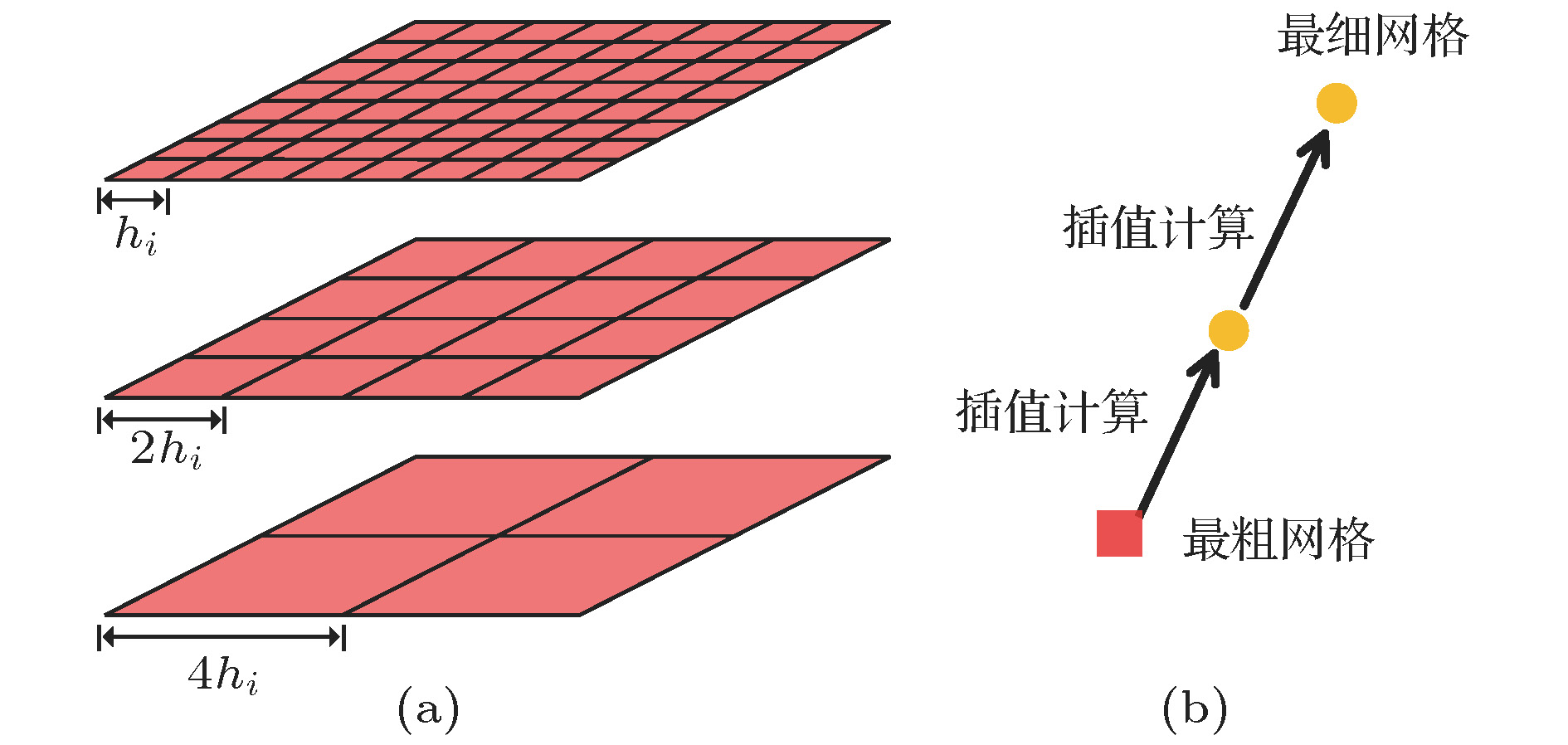
图 2 瀑布型多重网格法示意图　(a)网格结构; (b)CMG算法计算流程

Figure 2. Schematic of the CMG method: (a) Structure of network layers; (b) calculation process.

DownLoad: Full-Size Img PowerPoint

图 3 CMG算法降采样过程　(a)细网格上光场; (b)粗网格上光场

Figure 3. Downsampling process of the CMG method: (a) Data on the fine network; (b) data on the coarse network.

DownLoad: Full-Size Img PowerPoint

图 4 CMG算法插值过程　(a)细网格光场和粗网格光场的关系; (b)待插值数据位于正方形中心; (c), (d)待插值数据位于正方形四边上

Figure 4. Interpolation process of the CMG method: (a) The relationship between grid points on coarse network and fine network; (b) the new grid point located at the center of the unit square; (c), (d) the new grid point located on the edge of the unit square.

DownLoad: Full-Size Img PowerPoint

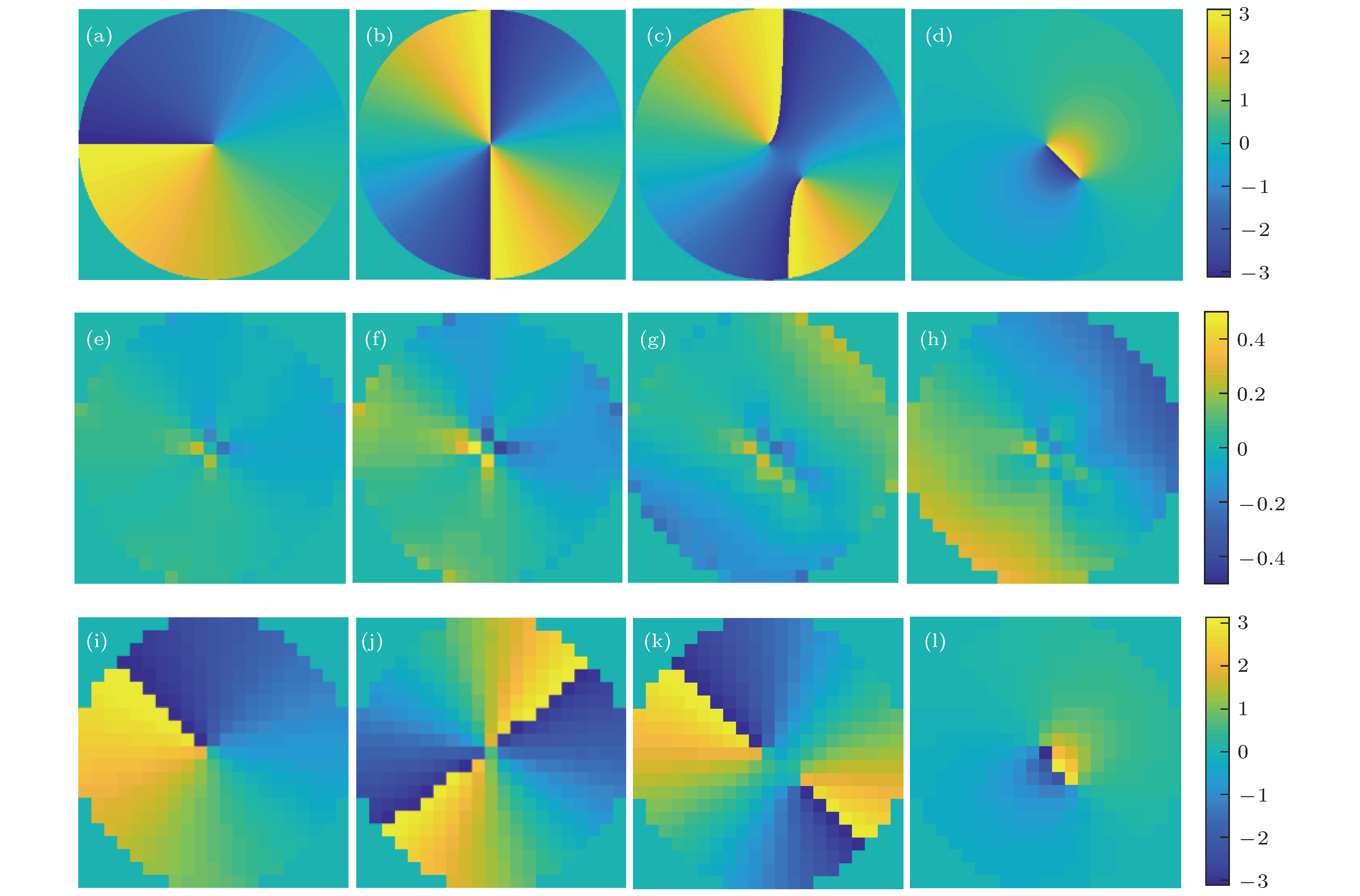
图 5 (a)−(d) Phase1, Phase2, Phase3和Phase4二维分布; (e)−(h)最小二乘法波前复原结果; (i)−(l)复指数波前复原算法结果

Figure 5. (a)−(d) Two-dimensional distribution of Phase1, Phase2, Phase3 and Phase4; (e)−(h) wavefront reconstructed by the least-squares reconstruction algorithm; (i)−(l) wavefront reconstructed by the CER algorithm.

DownLoad: Full-Size Img PowerPoint

图 6 直接迭代和CMG算法波前复原残差　(a)子孔径数目为20 × 20; (b)子孔径数目为40 × 40; (c)子孔径数目为80 × 80

Figure 6. Wavefront residual error of the direct iteration method and the CMG method, the number of subapertures is (a) 20 × 20; (b) 40 × 40; (c) 80 × 80.

DownLoad: Full-Size Img PowerPoint

图 7 CMG算法和直接迭代过程所需浮点乘运算数目(a)子孔径数目为20 × 20; (b)子孔径数目为40 × 40; (c)子孔径数目为80 × 80

Figure 7. Float point multiplications required by the CMG method and the process of the direct iteration the number of subapertures is (a) 20 × 20; (b) 40 × 40; (c) 80 × 80.

DownLoad: Full-Size Img PowerPoint

图 8 CMG算法和SOR算法波前复原残差统计结果

Figure 8. Wavefront residual statistics of the CMG method and SOR method.

DownLoad: Full-Size Img PowerPoint

图 9 变形镜驱动器和哈特曼波前传感器子孔径匹配关系

Figure 9. Matching relation between actuators of deformable mirror and subapertures of Shack-Hartmann sensor.

DownLoad: Full-Size Img PowerPoint

图 10 不同Rytov方差时, 自适应光学系统校正前后远场光强分布及其峰值Strehl比

Figure 10. Far field intensity and Strehl ratio of laser beam before and after corrected by the adaptive optics system.

DownLoad: Full-Size Img PowerPoint

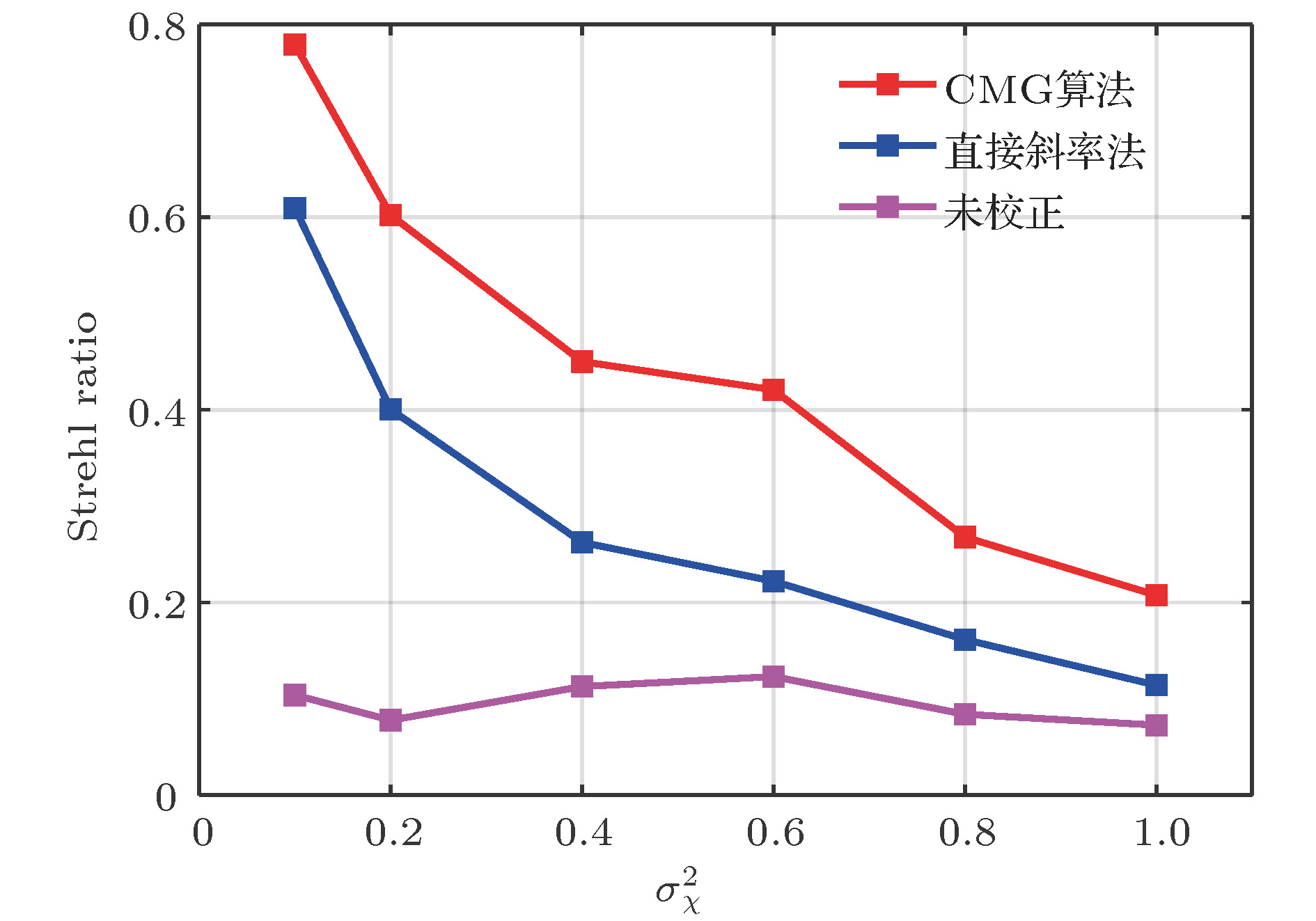
图 11 不同Rytov方差时, 自适应光学系统校正光束Strehl比

Figure 11. Strehl ratio of laser beam after corrected by the adaptive optics system in different Rytov number.

DownLoad: Full-Size Img PowerPoint

表 1 直接迭代和CMG算法波前复原时间(单位: s)

Table 1. Time required by the direct iteration and CMG method (in s).

	子孔径数目20 × 20		子孔径数目40 × 40		子孔径数目80 × 80
	直接迭代	CMG算法	直接迭代	CMG算法	直接迭代	CMG算法
Phase1	4.261	0.081	67.39	0.271	1400	0.920
Phase2	5.112	0.119	77.61	0.319	2134	0.852
Phase3	4.184	0.103	54.56	0.519	1424	1.339
Phase4	1.891	0.097	18.43	0.494	370.8	1.308

DownLoad: CSV

[1]	Fried D L, Vaughn J L 1992 Appl. Opt. 31 2865 Google Scholar
[2]	Fried D L 1998 JOSA A 15 2759 Google Scholar
[3]	Primmerman C A, Price T R, Humphreys R A, et al. 1995 Appl. Opt. 34 2081 Google Scholar
[4]	Lukin V P, Fortes B V 2002 Appl. Opt. 41 5616 Google Scholar
[5]	Steinbock M J, Hyde M W, Schmidt J D 2014 Appl. Opt. 53 3821 Google Scholar
[6]	Le B E, Wild W J, Kibblewhite E J 1998 Opt. Lett. 23 10 Google Scholar
[7]	Fried D L 2001 Opt. Commun. 200 43 Google Scholar
[8]	Barchers J D, Fried D L, Link D J 2002 Appl. Opt. 41 1012 Google Scholar
[9]	Aubailly M, Vorontsov M A 2012 JOSA A 29 1707
[10]	Yazdani R, Fallah H 2017 Appl. Opt. 56 1358 Google Scholar
[11]	Goodman J W ( translated by Qin K C, L P S, Chen J B, Cao Q Z) 2013 Introduction to Fourier Optics (3rd Ed.) (Beijing: Publishing House of Electronics Industry) p77
[12]	Hudgin R H 1977 JOSA 67 378 Google Scholar
[13]	Hudgin R H 1977 JOSA 67 375 Google Scholar
[14]	Bornemann F A, Deuflhard P 1996 Numerische Mathematik 75 135 Google Scholar
[15]	Venema T M, Schmidt J D 2008 Opt. Express 16 6985 Google Scholar
[16]	Steinbock M J, Schmidt J D, Hyde M W 2012 Aerospace Conference Big Sky, MT, USA, 3-10 March, 2012, pp1-13
[17]	Roddier N A 1990 Opt. Eng. 29 1174 Google Scholar
[18]	Southwell W H 1980 JOSA 70 998 Google Scholar
[19]	Jr J A F, Morris J R, Feit M D 1976 Appl. Phys. 10 129
[20]	蔡冬梅, 王昆, 贾鹏, 王东, 刘建霞 2014 物理学报 63 104217 Google Scholar Cai D M, Wang K, Jia P, Wang D, Liu J X 2014 Acta Phys. Sin. 63 104217 Google Scholar
[21]	程生毅, 陈善球, 董理治, 王帅, 杨平, 敖明武, 许冰 2015 物理学报 64 094207 Google Scholar Cheng Y C, Shan Q C, Dong L Z, Wang S, Yang P, Ao M W, Xu B 2015 Acta Phys. Sin. 64 094207 Google Scholar
[22]	Fan C, Wang Y, Gong Z 2004 Appl. Opt. 43 4334 Google Scholar

[1]	Zhao Ting, Gong Mao-Mao, Zhang Song-Bin. Theoretical study on photo-ionization of helium atoms by Bessel vortex light. Acta Physica Sinica, 2024, 73(24): 244201. doi: 10.7498/aps.73.20241378
[2]	Chen Ke-Le, Zhou Jia-Hui, Han Wen-Yu, Rao Xue-Jun, Guo You-Ming, Rao Chang-Hui. Fast estimation method of optimal modal gain for adaptive optical system. Acta Physica Sinica, 2023, 72(13): 139502. doi: 10.7498/aps.72.20230290
[3]	He Ting, Tian Bo-Yu, Qiu Die, Zhang Bin. Novel method of improving beam quality of thin-wall tube laser based on right-angle cone deformable mirror. Acta Physica Sinica, 2021, 70(17): 179501. doi: 10.7498/aps.70.20210603
[4]	Zhang Yan-Yan, Chen Su-Ting, Ge Jun-Xiang, Wan Fa-Yu, Mei Yong, Zhou Xiao-Yan. Removal of additive noise in adaptive optics system based on adaptive nonconvex sparse regularization. Acta Physica Sinica, 2017, 66(12): 129501. doi: 10.7498/aps.66.129501
[5]	Liu Zhang-Wen, Li Zheng-Dong, Zhou Zhi-Qiang, Yuan Xue-Wen. Adaptive optics correction technique based onfuzzy control. Acta Physica Sinica, 2016, 65(1): 014206. doi: 10.7498/aps.65.014206
[6]	Tang Yan-Qiu, Sun Qiang, Zhao Jian, Yao Kai-Nan. A closed-loop aberration compensating method of optics system based on holography. Acta Physica Sinica, 2015, 64(2): 024206. doi: 10.7498/aps.64.024206
[7]	Guo You-Ming, Rao Chang-Hui, Bao Hua, Zhang Ang, Wei Kai. Direct computation of the interaction matrix of adaptive optical system. Acta Physica Sinica, 2014, 63(14): 149501. doi: 10.7498/aps.63.149501
[8]	Guo You-Ming, Ma Xiao-Yu, Rao Chang-Hui. Optimal closed-loop bandwidth of tip-tilt correction loop in adaptive optics system. Acta Physica Sinica, 2014, 63(6): 069502. doi: 10.7498/aps.63.069502
[9]	Wang Yu-Yu, Gao Yan-Qi, Zhu Hai-Dong, Lu Xing-Hua, Zhang Jun-Yong, Guo Ya-Jing, Hui Hong-Chao, Zhu Bao-Qiang. Auto-alignment in four-pass amplifier with wavefront correction system. Acta Physica Sinica, 2013, 62(5): 055201. doi: 10.7498/aps.62.055201
[10]	Liu Chao, Hu Li-Fa, Mu Quan-Quan, Cao Zhao-Liang, Hu Hong-Bin, Zhang Xing-Yun, Lu Yong-Jun, Xuan Li. Modal prediction for open-loop liquid-crystal adaptive optics systems. Acta Physica Sinica, 2012, 61(12): 129501. doi: 10.7498/aps.61.129501
[11]	Liu Chao, Hu Li-Fa, Cao Zhao-Liang, Mu Quan-Quan, Peng Zeng-Hui, Xuan Li. Dynamic wavefront correction with a fast liquid-crystal on silicon device of pure phase. Acta Physica Sinica, 2012, 61(8): 089501. doi: 10.7498/aps.61.089501
[12]	Jian Xiao-Hua, Cui Yao-Yao, Xiang Yong-Jia, Han Zhi-Le. Adaptive optics multispectral photoacoustic imaging. Acta Physica Sinica, 2012, 61(21): 217801. doi: 10.7498/aps.61.217801
[13]	Lu Jing, Li Hao, He Yi, Shi Guo-Hua, Zhang Yu-Dong. Superresolution in adaptive optics confocal scanning laser ophthalmoscope. Acta Physica Sinica, 2011, 60(3): 034207. doi: 10.7498/aps.60.034207
[14]	Wang Jian-Xin, Bai Fu-Zhong, Ning Yu, Huang Lin-Hai, Jiang Wen-Han. Diffraction theory analysis and numerical simulation of non-modulation two-sided pyramid wavefront sensor. Acta Physica Sinica, 2011, 60(2): 029501. doi: 10.7498/aps.60.029501
[15]	Zhang Yan-Yan, Rao Chang-Hui, Li Mei, Ma Xiao-Yu. The detection error analysis of Hartmann-Shack wavefront sensor based on electron multiplying charge-coupled devices. Acta Physica Sinica, 2010, 59(8): 5904-5913. doi: 10.7498/aps.59.5904
[16]	Bai Fu-Zhong, Rao Chang-Hui. Effect of pinhole diameter on measurement accuracy of self-referencing interferometer wavefront sensor. Acta Physica Sinica, 2010, 59(6): 4056-4064. doi: 10.7498/aps.59.4056
[17]	Bai Fu-Zhong, Rao Chang-Hui. Effect of pinhole diameter on correction accuracy of closed-loop adaptive optics system using self-referencing interferometer wavefront sensor. Acta Physica Sinica, 2010, 59(11): 8280-8286. doi: 10.7498/aps.59.8280
[18]	Ning Yu, Yu Hao, Zhou Hong, Rao Chang-Hui, Jiang Wen-Han. Performance test and closed-loop correction experiment of a 20-element bimorph deformable mirror. Acta Physica Sinica, 2009, 58(7): 4717-4723. doi: 10.7498/aps.58.4717
[19]	Cai Dong-Mei, Ling Ning, Jiang Wen-Han. The performance of phase-only liquid crystal spatial light modulator used for generating Zernike terms. Acta Physica Sinica, 2008, 57(2): 897-903. doi: 10.7498/aps.57.897
[20]	Li Chao-Hong, Xian Hao, Jiang Wen-Han, Rao Chang-Hui. Analysis of wavefront measuring method for daytime adaptive optics. Acta Physica Sinica, 2007, 56(7): 4289-4296. doi: 10.7498/aps.56.4289

期刊类型引用(1)
1. 韩冰冰. 基于矩形有限元离散泊松方程的二重网格法研究. 安阳师范学院学报. 2021(05): 5-8 . 百度学术
其他类型引用(1)

Catalog

Vol. 68, Issue 10 - 2019-05-20

Metrics

Abstract views: 8214
PDF Downloads: 43
Cited By: 2

姓名
邮箱
手机号码
标题
留言内容
验证码

Search

Article

留言板