Quantum image chaos encryption scheme based on quantum long-short term memory network

Wang Wei-Jie; Jiang Mei-Mei; Wang Shu-Mei; Qu Ying-Jie; Ma Hong-Yang; Qiu Tian-Hui

doi:10.7498/aps.72.20230242

Abstract

In recent years, the transmission security of image information has become an important research direction in the internet field. In this work, we propose a quantum image chaos encryption scheme based on quantum long-short term memory (QLSTM) network. We find that because the QLSTM network has a complex structure and more parameters, when the QLSTM network is used to improve the Lorenz chaotic sequence, its largest Lyapunov exponent is 2.5465% higher than that of the original sequence and 0.2844% higher than that the sequence improved by the classical long-short term memory (LSTM) network, while its result is closer to 1 and more stable in the 0–1 test. The improved sequence of QLSTM network has better chaotic performance and is predicted more difficultly, which improves the security of single chaotic system encryption. The original image is stored in the form of quantum states by using the NCQI quantum image representation model, and the improved sequence of QLSTM network is used to control the three-level radial diffusion, quantum generalized Arnold transform and quantum W-transform respectively, so that the gray value and pixel position of the quantum image are changed and the final encrypted image is obtained. The encryption scheme proposed in this work obtains the average information entropy of all three channels of RGB of greater than 7.999, the average value of pixel number change rate of 99.6047%, the average value of uniform average change intensity of 33.4613%, the average correlation of 0.0038, etc. In the test of statistical properties, the encryption scheme has higher security than some other traditional methods and can resist the common attacks.

Keywords:

quantum image encryption /
quantum long-short term memory network /
chaotic systems

Authors and contacts

School of Science, Qingdao University of Technology, Qingdao 266520, China

Corresponding author: Qiu Tian-Hui, qiutianhui@qut.edu.cn

Funds: Project supported by the Natural Science Foundation of Shandong Province, China (Grant No. ZR2021MF049), the Joint Fund of Natural Science Foundation of Shandong Province, China (Grant Nos. ZR2022LLZ012, ZR2021LLZ001), the Innovation and Entrepreneurship Training Program for College Students of Shandong Province, China (Grant No. S202210429001), and the Scientific and Technological Innovation Project for College Students of Qingdao University of Technology, China (Grant No. KJCXXM141)

FullText HTML : translate this paragraph

References

[1]	Shakir H R, Mehdi S A A, Hattab A A 2022 Bull. Electr. Eng. Inform. 11 2645 Google Scholar
[2]	王一诺, 宋昭阳, 马玉林, 华南, 马鸿洋 2021 物理学报 70 230302 Google Scholar Wang Y N, Song Z Y, Ma Y L, Hua N, Ma H Y 2021 Acta Phys. Sin. 70 230302 Google Scholar
[3]	Liu G Z, Li W, Fan X K, Li Z, Wang Y X, Ma H Y 2022 Entropy 24 608 Google Scholar
[4]	Zhao J B, Zhang T, Jiang J W, Fang T, Ma H Y 2022 Sci. Rep. 12 14253 Google Scholar
[5]	Li C Q, Lin D D, Lu J H 2017 IEEE MultiMedia 24 64 Google Scholar
[6]	Li C M, Yang X Z 2022 Optik 260 169042 Google Scholar
[7]	Xian Y J, Wang X Y 2021 Inf. Sci. 547 1154 Google Scholar
[8]	Zhou N R, Hu Y Q, Gong L H, Li G Y 2017 Quantum Inf. Process. 16 164 Google Scholar
[9]	Liu H, Zhao B, Huang L Q 2019 Entropy 21 343 Google Scholar
[10]	Song X H, Wang S, Abd El-Latif A A, Niu X M 2014 Quantum Inf. Process. 13 1765 Google Scholar
[11]	Akhshani A, Akhavan A, Lim S C, Hassan Z 2012 Commun. Nonlinear Sci. Numer. Simul. 17 4653 Google Scholar
[12]	Zhou N R, Huang L X, Gong L H, Zeng Q W 2020 Quantum Inf. Process. 19 284 Google Scholar
[13]	Wang X Y, Su Y I, Luo C, Nian F Z, Teng L 2022 Multimedea Tools Appl. 81 13845 Google Scholar
[14]	Gao Y J, Xie H W, Zhang J, Zhang H 2022 Physia A 598 127334 Google Scholar
[15]	Liu X B, Xiao D, Liu C 2021 Quantum Inf. Process. 20 23 Google Scholar
[16]	Jiang J W, Zhang T, Li W, Wang S M 2023 Quantum Eng. 2023 3746357 Google Scholar
[17]	Zhao J F, Wang S Y, Chang Y X, Li X F 2015 Nonlinear Dyn. 80 1721 Google Scholar
[18]	Chai X L, Fu J Y, Zhang J T, Han D J, Gan Z H 2021 Neural. Comput. Appl. 33 10371 Google Scholar
[19]	Chai X L, Gan Z H, Yuan K, Lu Y, Chen Y R 2017 Chin. Phys. B 26 020504 Google Scholar
[20]	Jiang N, Dong X, Hu H, Ji Z X, Zhang W Y 2019 Int. J. Theor. Phys. 58 979 Google Scholar
[21]	Ge B, Luo H B 2020 Int. J. Autom. Comput. 17 123 Google Scholar
[22]	Hu W B, Dong Y M 2022 J. Appl. Phys. 131 114402 Google Scholar
[23]	刘瀚扬, 华南, 王一诺, 梁俊卿, 马鸿洋 2022 物理学报 71 170303 Google Scholar Liu H Y, Hua N, Wang Y N, Liang J Q, Ma H Y 2022 Acta Phys. Sin. 71 170303 Google Scholar
[24]	Faqih A, Kamanditya B, Kusumoputro B 2018 International Conference on Computer, Information and Telecommunication Systems (Alsace: IEEE) p1
[25]	Qu J Y, Zhao T, Ye M, Li J Y, Liu C 2020 Neural Process. Lett. 52 1461 Google Scholar
[26]	Yang G C, Zhu T, Wang H, Yang F B 2021 IEEE Trans. Circuits Syst. Express Briefs 69 1487 Google Scholar
[27]	Li Y T, Li Y 2022 Neurocomputing 491 321 Google Scholar
[28]	Li W, Chu P C, Liu G Z, Tian Y B, Qiu T H, Wang S M 2022 Quantum Eng. 2022 5701479 Google Scholar
[29]	Chen G M, Long S, Yuan Z D, Li W Y, Peng J F 2023 Quantum Eng. 2023 2842217 Google Scholar
[30]	Zhang Y, Ni Q 2021 Quantum Eng. 3 e75 Google Scholar
[31]	Wei S J, Chen Y H, Zhou Z R, Long G L 2022 AAPPS Bulletin 32 2 Google Scholar
[32]	Hochreiter S, Schmidhuber J 1997 Neural Comput. 9 1735 Google Scholar
[33]	Kandala A, Mezzacapo A, Temme K, Takita M, Brink M, Chow J M, Gambetta J M 2017 Nature 549 242 Google Scholar
[34]	McClean J R, Romero J, Babbush R, Aspuru-Guzik A 2016 New J. Phys. 18 023023 Google Scholar
[35]	Chen S Y C, Yang C H H, Qi J, Chen P Y, Ma X L, Goan H S 2020 IEEE Access 8 141007 Google Scholar
[36]	Schuld M, Bocharov A, Svore K M, Wiebe N 2020 Phys. Rev. A 101 032308 Google Scholar
[37]	Benedetti M, Lloyd E, Sack S, Fiorentini M 2019 Quantum Sci. Technol. 4 043001 Google Scholar
[38]	Havlicek V, Corcoles A D, Temme K, Harrow A W, Kandala A, Chow J M, Gambetta J M 2019 Nature 567 209 Google Scholar
[39]	Di Sipio R, Huang J H, Chen S Y C, Mangini S, Worring M 2022 ICASSP 2022–2022 IEEE International Conference on Acoustics, Speech and Signal Processing (Singapore: IEEE) p8612
[40]	Sang J Z, Wang S, Li Q 2017 Quantum Inf. Process. 16 42 Google Scholar
[41]	Wu Y L 2008 Electron. Sci. 21 69
[42]	Wolf A, Swift J B, Swinney H L, Vastano J A 1985 Phys. D: Nonlinear Phenomena 16 285 Google Scholar
[43]	赵智鹏, 周双, 王兴元 2021 物理学报 70 230502 Google Scholar Zhao Z P, Zhou S, Wang X Y 2021 Acta Phys. Sin. 70 230502 Google Scholar
[44]	Gottwald G A, Melbourne I 2004 Proc. R. Soc. London, Ser. A 460 603 Google Scholar
[45]	Sun K H, Liu X, Zhu C X 2010 Chin. Phys. B 19 110510 Google Scholar
[46]	Boriga R, Dascalescu A C, Priescu I 2014 Signal Process. Image Commun. 29 887 Google Scholar
[47]	Raja S S, Mohan V 2014 Int. J. Adv. Eng. Res. 8 1
[48]	Yang Y G, Tian J, Lei H, Zhou Y H, Shi W M 2016 Inf. Sci. 345 257 Google Scholar

Cited By

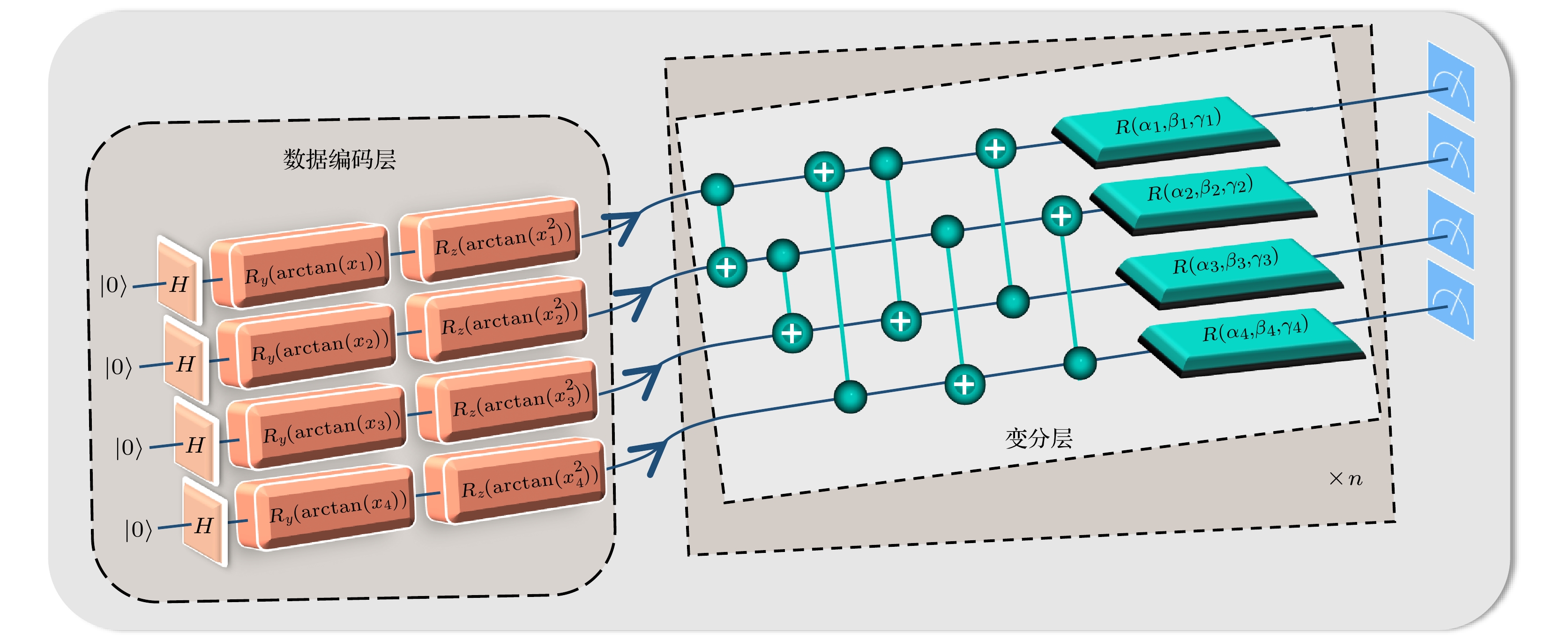
图 1 VQC的通用架构

Figure 1. General architecture of VQC

DownLoad: Full-Size Img PowerPoint

图 2 QLSTM网络的循环单元结构

Figure 2. Cyclic cell structure of QLSTM network

DownLoad: Full-Size Img PowerPoint

图 3 径向扩散　(a)原序列; (b)二位径向扩散; (c)四位径向扩散; (d) 八位径向扩散

Figure 3. Radial diffusion: (a) Original sequence; (b) two-position radial diffusion; (c) four-position radial diffusion; (d) eight-position radial diffusion

DownLoad: Full-Size Img PowerPoint

图 4 LSTM网络和QLSTM网络改进的序列的LLE曲线

Figure 4. Largest Lyapunov exponent curves for sequences improved by LSTM network or QLSTM network

DownLoad: Full-Size Img PowerPoint

图 5 Lorenz混沌序列、LSTM网络和QLSTM网络改进的序列的0—1测试图

Figure 5. 0–1 test images for Lorenz chaotic sequences and sequences improved by LSTM network or QLSTM network

DownLoad: Full-Size Img PowerPoint

图 6 加密和解密的效果图

Figure 6. Effect of encryption and decryption

DownLoad: Full-Size Img PowerPoint

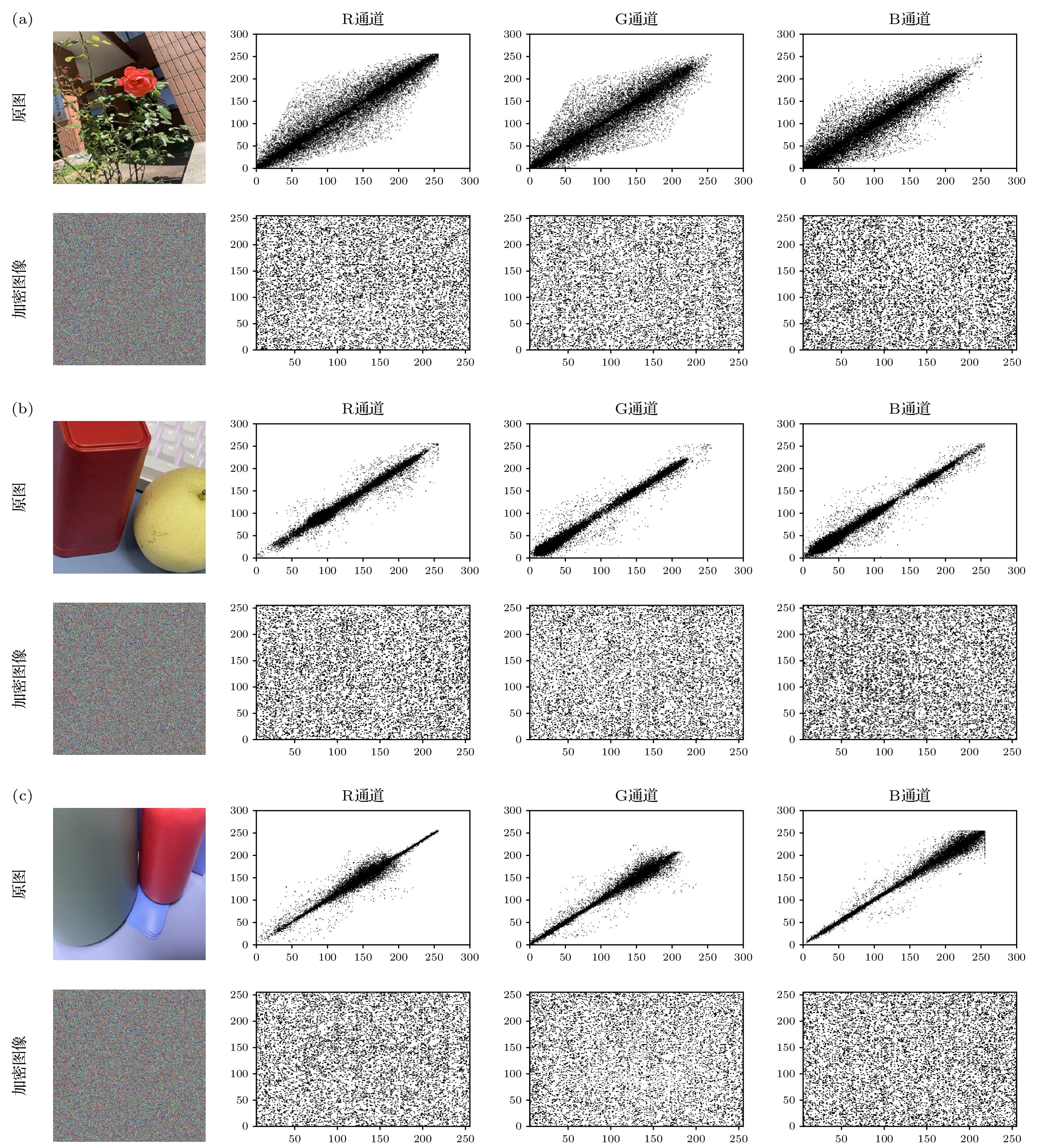
图 7 加密前后相关性分析对比图

Figure 7. Comparison of pixel correlation analysis before and after encryption

DownLoad: Full-Size Img PowerPoint

图 8 加密前后直方图分析对比图

Figure 8. Comparison of histogram analysis before and after encryption

DownLoad: Full-Size Img PowerPoint

表 1 LLE数据对比

Table 1. Comparison of LLE data

序列来源	LLE
Henon映射	0.4192
超混沌Lorenz系统	0.3381
LSTM网络改进的序列^[43]	2.6002
QLSTM网络改进的序列	2.8846

DownLoad: CSV

表 2 0—1测试的数据对比

Table 2. Comparison of from 0–1 test data

序列来源	0—1测试
Henon映射^[45]	0.6173
超混沌Lorenz系统	0.7937
LSTM网络改进的序列^[43]	0.9218
QLSTM网络改进的序列	0.9572

DownLoad: CSV

表 3 加密图像的相关性分析

Table 3. Pixel correlation analysis of encrypted images

图像	通道	水平	垂直	对角
	R	0.0074	0.0031	0.0064
1	G	0.0039	0.0021	0.0019
	B	0.0044	0.0013	0.0058
	R	0.0006	0.0067	0.0026
2	G	0.0017	0.0049	0.0047
	B	0.0057	0.0006	0.0069
	R	0.0003	0.0052	0.0013
3	G	0.0035	0.0005	0.0042
	B	0.0090	0.0029	0.0045

DownLoad: CSV

表 4 加密图像的信息熵

Table 4. Information entropy of encrypted images

图像	R	G	B
1	7.99928	7.99973	7.99951
2	7.99935	7.99908	7.99975
3	7.99912	7.99949	7.99921

DownLoad: CSV

表 5 加密图像的NPCR与UACI

Table 5. NPCR and UACI of encrypted images.

图像	NPCR	UACI
1	99.6048%	33.4604%
2	99.6063%	33.4609%
3	99.6029%	33.4627%

DownLoad: CSV

表 6 NPCR与UACI的对比分析

Table 6. Comparison of NPCR and UACI

算法	平均NPCR	平均UACI
本文	99.6047%	33.4613%
文献[43]	99.604%	33.46%

DownLoad: CSV

[1]	Shakir H R, Mehdi S A A, Hattab A A 2022 Bull. Electr. Eng. Inform. 11 2645 Google Scholar
[2]	王一诺, 宋昭阳, 马玉林, 华南, 马鸿洋 2021 物理学报 70 230302 Google Scholar Wang Y N, Song Z Y, Ma Y L, Hua N, Ma H Y 2021 Acta Phys. Sin. 70 230302 Google Scholar
[3]	Liu G Z, Li W, Fan X K, Li Z, Wang Y X, Ma H Y 2022 Entropy 24 608 Google Scholar
[4]	Zhao J B, Zhang T, Jiang J W, Fang T, Ma H Y 2022 Sci. Rep. 12 14253 Google Scholar
[5]	Li C Q, Lin D D, Lu J H 2017 IEEE MultiMedia 24 64 Google Scholar
[6]	Li C M, Yang X Z 2022 Optik 260 169042 Google Scholar
[7]	Xian Y J, Wang X Y 2021 Inf. Sci. 547 1154 Google Scholar
[8]	Zhou N R, Hu Y Q, Gong L H, Li G Y 2017 Quantum Inf. Process. 16 164 Google Scholar
[9]	Liu H, Zhao B, Huang L Q 2019 Entropy 21 343 Google Scholar
[10]	Song X H, Wang S, Abd El-Latif A A, Niu X M 2014 Quantum Inf. Process. 13 1765 Google Scholar
[11]	Akhshani A, Akhavan A, Lim S C, Hassan Z 2012 Commun. Nonlinear Sci. Numer. Simul. 17 4653 Google Scholar
[12]	Zhou N R, Huang L X, Gong L H, Zeng Q W 2020 Quantum Inf. Process. 19 284 Google Scholar
[13]	Wang X Y, Su Y I, Luo C, Nian F Z, Teng L 2022 Multimedea Tools Appl. 81 13845 Google Scholar
[14]	Gao Y J, Xie H W, Zhang J, Zhang H 2022 Physia A 598 127334 Google Scholar
[15]	Liu X B, Xiao D, Liu C 2021 Quantum Inf. Process. 20 23 Google Scholar
[16]	Jiang J W, Zhang T, Li W, Wang S M 2023 Quantum Eng. 2023 3746357 Google Scholar
[17]	Zhao J F, Wang S Y, Chang Y X, Li X F 2015 Nonlinear Dyn. 80 1721 Google Scholar
[18]	Chai X L, Fu J Y, Zhang J T, Han D J, Gan Z H 2021 Neural. Comput. Appl. 33 10371 Google Scholar
[19]	Chai X L, Gan Z H, Yuan K, Lu Y, Chen Y R 2017 Chin. Phys. B 26 020504 Google Scholar
[20]	Jiang N, Dong X, Hu H, Ji Z X, Zhang W Y 2019 Int. J. Theor. Phys. 58 979 Google Scholar
[21]	Ge B, Luo H B 2020 Int. J. Autom. Comput. 17 123 Google Scholar
[22]	Hu W B, Dong Y M 2022 J. Appl. Phys. 131 114402 Google Scholar
[23]	刘瀚扬, 华南, 王一诺, 梁俊卿, 马鸿洋 2022 物理学报 71 170303 Google Scholar Liu H Y, Hua N, Wang Y N, Liang J Q, Ma H Y 2022 Acta Phys. Sin. 71 170303 Google Scholar
[24]	Faqih A, Kamanditya B, Kusumoputro B 2018 International Conference on Computer, Information and Telecommunication Systems (Alsace: IEEE) p1
[25]	Qu J Y, Zhao T, Ye M, Li J Y, Liu C 2020 Neural Process. Lett. 52 1461 Google Scholar
[26]	Yang G C, Zhu T, Wang H, Yang F B 2021 IEEE Trans. Circuits Syst. Express Briefs 69 1487 Google Scholar
[27]	Li Y T, Li Y 2022 Neurocomputing 491 321 Google Scholar
[28]	Li W, Chu P C, Liu G Z, Tian Y B, Qiu T H, Wang S M 2022 Quantum Eng. 2022 5701479 Google Scholar
[29]	Chen G M, Long S, Yuan Z D, Li W Y, Peng J F 2023 Quantum Eng. 2023 2842217 Google Scholar
[30]	Zhang Y, Ni Q 2021 Quantum Eng. 3 e75 Google Scholar
[31]	Wei S J, Chen Y H, Zhou Z R, Long G L 2022 AAPPS Bulletin 32 2 Google Scholar
[32]	Hochreiter S, Schmidhuber J 1997 Neural Comput. 9 1735 Google Scholar
[33]	Kandala A, Mezzacapo A, Temme K, Takita M, Brink M, Chow J M, Gambetta J M 2017 Nature 549 242 Google Scholar
[34]	McClean J R, Romero J, Babbush R, Aspuru-Guzik A 2016 New J. Phys. 18 023023 Google Scholar
[35]	Chen S Y C, Yang C H H, Qi J, Chen P Y, Ma X L, Goan H S 2020 IEEE Access 8 141007 Google Scholar
[36]	Schuld M, Bocharov A, Svore K M, Wiebe N 2020 Phys. Rev. A 101 032308 Google Scholar
[37]	Benedetti M, Lloyd E, Sack S, Fiorentini M 2019 Quantum Sci. Technol. 4 043001 Google Scholar
[38]	Havlicek V, Corcoles A D, Temme K, Harrow A W, Kandala A, Chow J M, Gambetta J M 2019 Nature 567 209 Google Scholar
[39]	Di Sipio R, Huang J H, Chen S Y C, Mangini S, Worring M 2022 ICASSP 2022–2022 IEEE International Conference on Acoustics, Speech and Signal Processing (Singapore: IEEE) p8612
[40]	Sang J Z, Wang S, Li Q 2017 Quantum Inf. Process. 16 42 Google Scholar
[41]	Wu Y L 2008 Electron. Sci. 21 69
[42]	Wolf A, Swift J B, Swinney H L, Vastano J A 1985 Phys. D: Nonlinear Phenomena 16 285 Google Scholar
[43]	赵智鹏, 周双, 王兴元 2021 物理学报 70 230502 Google Scholar Zhao Z P, Zhou S, Wang X Y 2021 Acta Phys. Sin. 70 230502 Google Scholar
[44]	Gottwald G A, Melbourne I 2004 Proc. R. Soc. London, Ser. A 460 603 Google Scholar
[45]	Sun K H, Liu X, Zhu C X 2010 Chin. Phys. B 19 110510 Google Scholar
[46]	Boriga R, Dascalescu A C, Priescu I 2014 Signal Process. Image Commun. 29 887 Google Scholar
[47]	Raja S S, Mohan V 2014 Int. J. Adv. Eng. Res. 8 1
[48]	Yang Y G, Tian J, Lei H, Zhou Y H, Shi W M 2016 Inf. Sci. 345 257 Google Scholar

[1]	Yang Guang, Chao Su-Ya, Nie Min, Liu Yuan-Hua, Zhang Mei-Ling. Construction method of hybrid quantum long-short term memory neural network for image classification. Acta Physica Sinica, 2023, 72(5): 058901. doi: 10.7498/aps.72.20221924
[2]	Zhao Zhi-Peng, Zhou Shuang, Wang Xing-Yuan. A new chaotic signal based on deep learning and its application in image encryption. Acta Physica Sinica, 2021, 70(23): 230502. doi: 10.7498/aps.70.20210561
[3]	Fang Jie, Jiang Ming-Hao, An Xiao-Yu, Sun Jun-Wei. "One image corresponding to one key" image encryption algorithm based on chaotic encryption and DNA encoding. Acta Physica Sinica, 2021, 70(7): 070501. doi: 10.7498/aps.70.20201642
[4]	Wen He-Ping, Yu Si-Min, Lü Jin-Hu. Encryption algorithm based on Hadoop and non-degenerate high-dimensional discrete hyperchaotic system. Acta Physica Sinica, 2017, 66(23): 230503. doi: 10.7498/aps.66.230503
[5]	Wei De-Zhi, Chen Fu-Ji, Zheng Xiao-Xue. Internet public opinion chaotic prediction based on chaos theory and the improved radial basis function in neural networks. Acta Physica Sinica, 2015, 64(11): 110503. doi: 10.7498/aps.64.110503
[6]	Zhang Ling-Mei, Zhang Jian-Wen, Wu Run-Heng. Anti-control of Hopf bifurcation in the new chaotic system with piecewise system and exponential system. Acta Physica Sinica, 2014, 63(16): 160505. doi: 10.7498/aps.63.160505
[7]	Zhang Hong-Li, Song Li-Li. Parameter identification in chaotic systems by means of quantum particle swarm optimization. Acta Physica Sinica, 2013, 62(19): 190508. doi: 10.7498/aps.62.190508
[8]	Feng Chao-Wen, Cai Li, Kang Qiang, Zhang Li-Sen. A novel three-dimensional autonomous chaotic system. Acta Physica Sinica, 2011, 60(3): 030503. doi: 10.7498/aps.60.030503
[9]	Li Xiao-Hua, Liu Zhao-Hua, Zhang Ying-Jie, Zhang Jing, Wu Jian-Hui. ADRC and CMAC combined optimization and control for a class of discrete-time uncertain chaotic systems. Acta Physica Sinica, 2011, 60(3): 030701. doi: 10.7498/aps.60.030701
[10]	Tang Liang-Rui, Li Jing, Fan Bing, Zhai Ming-Yue. A new three-dimensional chaotic system and its circuit simulation. Acta Physica Sinica, 2009, 58(2): 785-793. doi: 10.7498/aps.58.785
[11]	Zhang Jian-Xiong, Tang Wan-Sheng, Xu Yong. A new three-dimensional chaotic system. Acta Physica Sinica, 2008, 57(11): 6799-6807. doi: 10.7498/aps.57.6799
[12]	Li Wen-Lin, Song Yun-Zhong. Chaos anti-control of nonlinear system with uncertainties. Acta Physica Sinica, 2008, 57(1): 51-55. doi: 10.7498/aps.57.51
[13]	Zhang Min, Hu Shou-Song. Adaptive control of uncertain chaotic systems with time delays using dynamic structure neural network. Acta Physica Sinica, 2008, 57(3): 1431-1438. doi: 10.7498/aps.57.1431
[14]	Yang Dong-Sheng, Zhang Hua-Guang, Li Ai-Ping, Meng Zi-Yi. Generalized synchronization of two non-identical chaotic systems based on fuzzy model. Acta Physica Sinica, 2007, 56(6): 3121-3126. doi: 10.7498/aps.56.3121
[15]	Luo Run-Zi. Impulsive control and synchronization of a new chaotic system. Acta Physica Sinica, 2007, 56(10): 5655-5660. doi: 10.7498/aps.56.5655
[16]	Niu Pei_Feng, Zhang Jun, Guan Xin_Ping. Research on a proportional-integral-derivative neural network decoupling control based on genetic algorithm optimization for unified chaotic system. Acta Physica Sinica, 2007, 56(5): 2493-2497. doi: 10.7498/aps.56.2493
[17]	Wang Jie-Zhi, Chen Zeng-Qiang, Yuan Zhu-Zhi. A new chaotic system and analysis of its properties. Acta Physica Sinica, 2006, 55(8): 3956-3963. doi: 10.7498/aps.55.3956
[18]	Lu Zhi-Gang, Yu Ling-Hui, Liu Xiao-Jing, Gao Mei-Jing, Wu Shi-Chang. . Acta Physica Sinica, 2002, 51(10): 2211-2215. doi: 10.7498/aps.51.2211
[19]	GUAN XIN-PING, FAN ZHENG-PING, PENG HAI-PENG, WANG YI-QUN. THE SYNCHRONIZATION OF CHAOTIC SYSTEMS BASED ON RBF NETWORK IN THE PRESENCE OF PERTURBATION. Acta Physica Sinica, 2001, 50(9): 1670-1674. doi: 10.7498/aps.50.1670
[20]	GUAN XIN-PING, TANG YING-GAN, FAN ZHENG-PING, WANG YI-QUN. NEURAL NERWORK BASED ROBUST ADAPTIVE SYNCHRONIZATION OF A CHAOTIC SYSTEM. Acta Physica Sinica, 2001, 50(11): 2112-2115. doi: 10.7498/aps.50.2112

Catalog

Vol. 72, Issue 12 - 2023-06-20

Metrics

Abstract views: 4068
PDF Downloads: 131
Cited By: 0

姓名
邮箱
手机号码
标题
留言内容
验证码

Search

Article

留言板