


-
Quantum scar is an intriguing phenomenon in quantum or wave dynamics that the wavefunction takes an exceptionally large value around an unstable periodic orbit. It has attracted much attention and advances the understanding of the semiclassical quantization. Most of previous researches involving quantum scars focus on hard-wall quantum billiards. Here we investigate the quantum billiard with a smooth confinement potential which possesses complex classical dynamics. We demonstrate that the semiclassical quantization approach works well for both the stable and unstable classical periodic orbit, besides the fact that the shape of the orbits varies as the energy increases or even the stability switches. The recurrence rule of the quantum scars in this complex solf-wall billiard differs from that of the hard-wall nonrelativistic quantum billiard, such as being equally spaced in energy instead of being equally spaced in the square root of energy. These results implement the previous knowledge and may be used for understanding the measurements of density of states and transport properties in two-dimensional electron systems with random long-range impurities.
-
Keywords:
- quantum scar /
- soft-wall quantum billiard /
- complex smooth potential quantum billiard /
- quantization rule
[1] Keller B J 1958 Ann. Phys. 4 180
 Google Scholar
[2] Einstein A 1917 Verh. Dtsch. Phys. Ges. 19 82
[3] Stone A D 2005 Phys. Today 58 37
Google Scholar
[4] Gutzwiller M C 1971 J. Math. Phys. 12 343
Google Scholar
[5] Cvitanovic P, Artuso R, Mainieri R, Tanner G, Vattay G, Whelan N, Wirzba A 2005 Chaos: Classical and Quantum (Copenhagen: Niels Bohr Institute) pp143–145
[6] Lichtenberg A J, Lieberman M A 1992 Regular and Chaotic Dynamics 2 nd edition (New York: SpringerVerlag) pp7–60
[7] Ott E 2002 Chaos in Dynamical Systems (2nd Ed.) (Cambridge: Cambridge University Press) pp421–450
[8] Knauf A, Sinai Y G 1997 Classical Nonintegrability, Quantum Chaos (Birkhuaser: Springer-Verlag) pp41–47
[9] Berry M V 1989 Phys. Scr. 40 335
Google Scholar
[10] Stöckmann H J 2006 Quantum Chaos: An Introduction (New York: Cambridge University Press) pp296–338
[11] Haake F 2010 Quantum Signatures of Chaos (3rd Ed.) (Berlin: Springer-Verlag) pp62–71
[12] Gutzwiller M C 2013 Chaos in Classical and Quantum Mechanics (New York: Springer-Verlag) pp116–118
[13] 徐躬耦 1995 量子混沌运动 (上海: 上海科学技术出版社) 第58—69页
Xu G O 1995 Quantum Chaotic Motions in Quantum Systems (Shanghai: Shanghai Scientific and Technical Publishers) pp58–69
[14] 顾雁 1996 量子混沌 (上海: 上海科学技术出版社) 第69—153页
Gu Y 1996 Quantum Chaos (Shanghai: Shanghai Scientific and Technological Education Publishing House) pp69–153
[15] Casati G and Chirikov B 2006 Quantum Chaos: Between Order and Disorder (New York: Cambridge University Press) pp317–385
[16] McDonald S W, Kaufman A N 1979 Phys. Rev. Lett. 42 1189
Google Scholar
[17] Heller E J 1984 Phys. Rev. Lett. 53 1515
Google Scholar
[18] McDonald S W, Kaufman A N 1988 Phys. Rev. A 37 3067
Google Scholar
[19] Bogomolny E B 1988 Physica D 31 169
Google Scholar
[20] Berry M V 1989 Proc. R. Soc. London, Ser. A 423 219
Google Scholar
[21] Agam O, Fishman S 1993 J. Phys. A Math. Gen. 26 2113
Google Scholar
[22] Agam O, Fishman S 1994 Phys. Rev. Lett. 73 806
Google Scholar
[23] Kroetz T, Oliveira H A, Portela J S E, Viana R L 2016 Phys. Rev. E 94 022218
Google Scholar
[24] Luukko P J J, Drury B, Klales A, Kaplan L, Heller E J, Räsänen E 2016 Sci. Rep. 6 37656
Google Scholar
[25] Keski-Rahkonen J, Luukko P J J, Kaplan L, Heller E J, Räsänen E 2017 Phys. Rev. B 96 094204
Google Scholar
[26] Keski-Rahkonen J, Ruhanen A, Heller E J, Räsänen E 2019 Phys. Rev. Lett. 123 214101
Google Scholar
[27] Keski-Rahkonen J, Luukko P J J, Åberg S, Räsänen E 2019 J. Phys. Condens. Matter 31 105301
Google Scholar
[28] Eckhardt B 1988 Phys. Rep. 163 205
Google Scholar
[29] Huang L, Lai Y C, Ferry D K, Goodnick S M, Akis R 2009 Phys. Rev. Lett. 103 054101
Google Scholar
[30] Xu H Y, Huang L, Lai Y C, Grebogi C 2013 Phys. Rev. Lett. 110 064102
Google Scholar
[31] Arnol'd V I 2013 Mathematical Methods of Classical Mechanics (New York: Springer Science & Business Media) pp30–50
[32] Miller W H 1975 J. Chem. Phys. 63 996
Google Scholar
[33] Voros A 1988 J. Phys. A: Math. Gen. 21 685
Google Scholar
[34] Huang L, Lai Y C, Luo H G, Grebogi C 2015 AIP Adv. 5 017137
Google Scholar
[35] Zhang G Q, Chen X, Lin L, Peng H, Liu Z, Huang L, Kang N, Xu H Q 2020 Phys. Rev. B 101 085404
Google Scholar
-
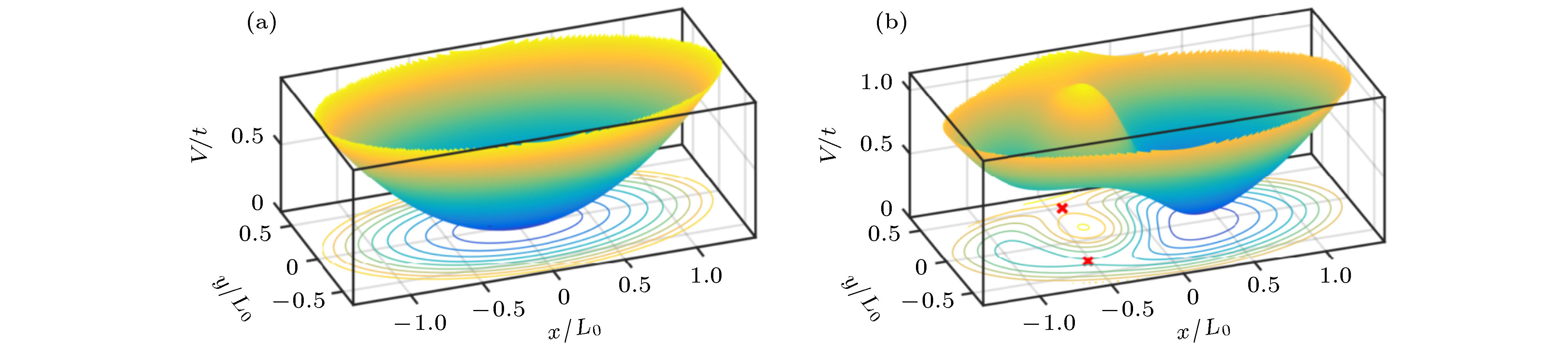
图 1 (a)二维谐振子势 ((2)式), 其中
$ L_0 $ 是系统的特征尺度,$ \omega'_x L_0 /(\sqrt{2}a) = 1 $ ,$ \omega'_y = 2\omega'_x $ . 为了破坏对称性, 我们在$ (x_{\delta}/L_0, y_{\delta}/L_0) = (-0.278, -0.226) $ 处加了一个$ \delta(x-x_0, y-y_0) $ 函数势; (b)在势场(a)的基础上, 加入了一个高斯势场$ V_{\rm G} = U{\rm e}^{-[(x-x_{\rm G})^2+(y-y_{\rm G})^2]/(2\sigma^2)} $ , 其中$ U = 1 t $ ,$ \sigma/L_0 = 0.2828 $ ,$ (x_{\rm G}/L_0, y_{\rm G}/L_0) = (-0.3441, 0.1226) $ . 这样整个势场形成左右两个谷, 一个峰, 其中右侧谷底的位置为$ (x_{\rm V}/L_0, y_{\rm V}/L_0) = (0.3574, -0.0179) $ , 对应的势能为$ V_{\min} = 0.1053 t $ . 两个势谷之间存在两个鞍点, 如叉号所标示的位置, 对应的势能分别为0.591t和0.976tFig. 1. (a) Two-dimensional harmonic potential (Eq. (2)), where
$ L_0 $ is the character scale of the system,$ \omega'_x L_0 /(\sqrt{2}a) = 1 $ , and$ \omega'_y = 2\omega'_x $ . To break the discrete symmetry, we added a$ \delta(x-x_0, y-y_0) $ potential at$ (x_{\delta}/L_0, y_{\delta}/L_0) = (-0.278, -0.226) $ ; (b) On the potential given in Fig.(a), we added an additional Gaussian potential$ V_{\rm G} = U{\rm e}^{-[(x-x_{\rm G})^2+(y-y_{\rm G})^2]/(2\sigma^2)} $ , where$ U = 1 t $ ,$ \sigma/L_0 = 0.2828 $ , and$ (x_{\rm G}/L_0, y_{\rm G}/L_0) = (-0.3441, 0.1226) $ . Thus the potential field forms two valleys and one peak, and the position of the bottom of the right valley is$ (x_{\rm V}/L_0, y_{\rm V}/L_0) = (0.3574, -0.0179) $ , with corresponding potential$ V_{\min} = 0.1053 t $ . There are two saddle points between the two valleys, as marked by the crosses, with corresponding potential values 0.591t and 0.976t.
图 2 图1(b)势场的庞加莱截面, 即
$ p_{\bot} = 0 $ 时$ p_{//} $ 对于此时的位置相对于右侧谷底的角度$ \theta $ ((a)—(c))和后面所处理的6 类轨道(d). (a)总能量$ E = 0.3 t $ ; (b)$ E = 0.45 t $ ; (c)$ E = 0.75 t $ Fig. 2. The Poincaré section of the motion of a particle moving in the potential field given by Fig. 1(b), e.g., when
$ p_{\bot} = 0 $ ,$ p_{//} $ vs. the angle$ \theta $ of this point with respect to the bottom of the right valley$ (x_{\rm V}, y_{\rm V}) $ ((a)–(c)). The total energy of the particle is$ E = 0.3 t $ (a),$ E = 0.45 t $ (b), and$ E = 0.75 t $ (c), respectively. (d) The six classes periodic orbits that will be discussed later.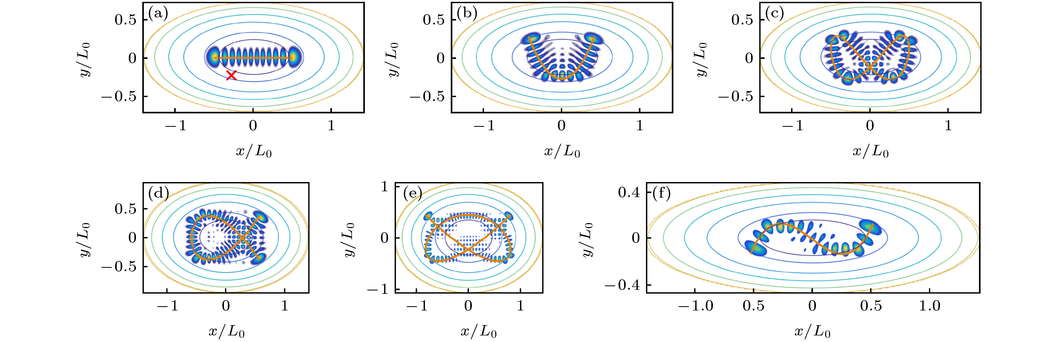
图 3 图1(a)势场下粒子的本征态. 图中所画为一些具有代表性的波函数的模方, 凝聚在李萨如轨道上.
$ x $ 和$ y $ 方向的频率比为(a)—(c) 1∶2, (d) 2∶3, (e) 3∶4, (f) 1∶3. 对所有情况,$ \omega'_x L_0 /\sqrt{2}a = 1 $ ,$ x/L_0 $ 的范围为$ [-\sqrt{2}, \sqrt{2}]L_0 $ , 谐振子势在$ y = 0 $ 的边界上的值为$ 1 t $ Fig. 3. The representative eigen-wavefunctions of the billiard Fig. 1(a). Shown are the the square of the modulus of wavefunctions that are condensed on the Lissajous orbits. The ratio of the frequency in
$ x $ and$ y $ directions are: (a)–(c) 1∶2, (d) 2∶3, (e) 3∶4, (f) 1∶3. For all case,$ \omega'_x L_0 /\sqrt{2}a = 1 $ , the range of$ x $ is$ [-\sqrt{2}, \sqrt{2}]L_0 $ and the value of the harmonic potential at the$ y = 0 $ boundary is$ 1t $ .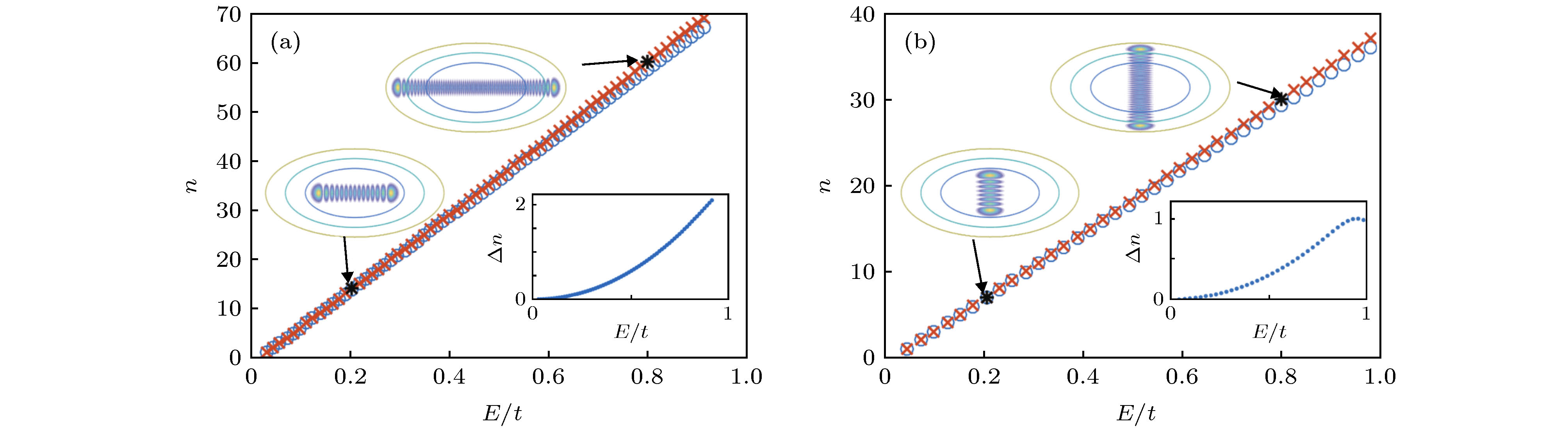
图 4 小扰动下二维谐振子势中的bouncing ball量子态的轨道方向量子数
$ n $ 对能量的依赖图. 叉号为根据波函数数出来的波长数减1, 圆圈为根据半经典公式得到的$ n $ (a)横向bouncing ball态; (b)纵向bouncing ball态. 小图$ \Delta n $ 为根据波函数数出来的结果和根据本征能量计算出来的结果的差Fig. 4. The quantum numbers
$ n $ along the trajectory vs. energy for bouncing ball states in the harmonic potential with a small perturbation. Crosses are the numbers of wavelengthes counted from the wavefunctions minus one, circles are derived from the semiclassical formulas: (a) Horizontal bouncing ball orbits; (b) vertical bouncing ball orbits. Insets show the difference$ \Delta n $ between these two methods.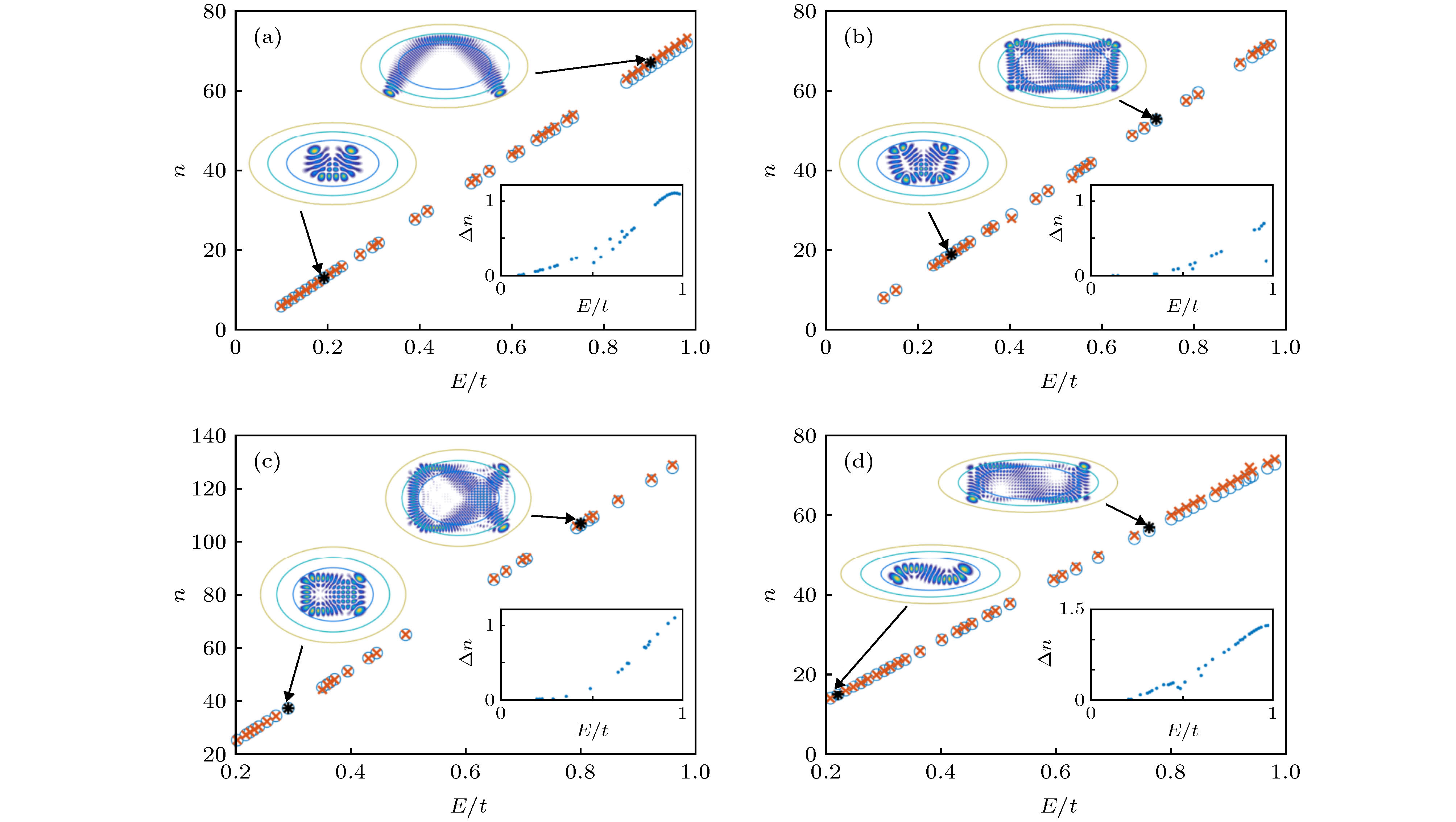
图 5 小扰动二维谐振子势场中4类李萨如态的量子化条件. 叉号为根据波函数数出来的波长数减1, 圆圈为根据半经典公式得到的
$ n $ . 图中小图为根据波函数数出来的结果和根据本征能量计算出来的结果的差Fig. 5. The quantization condition for the four types of scars for the harmonic potential with a small perturbation. Crosses are the numbers of wavelengthes counted from the wavefunctions minus one, circles are the quantum numbers derived from the semiclassical formulas. Insets show the difference
$ \Delta n $ between these two methods.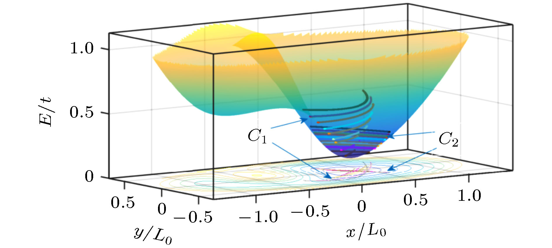
图 6 大扰动二维谐振子势场中的两类bouncing ball 轨道以及它们在零能量面上的投影. 纵轴对应的是每个轨道的能量值. 为了便于辨认, 势函数及其等势线也一起画在了图上. 第一组(C1)轨道对应着图2中在
$ p_{//} = 0 $ ,$ \theta/(2{\text{π}})\approx 0.1 $ 和$ 0.6 $ 处两个最显著的KAM岛的中心轨道, 第二组(C2)轨道对应着图2(a)中在$ p_{//} = 0 $ ,$ \theta/(2{\text{π}})\approx $ 0.33和0.86 处两个KAM岛的中心轨道Fig. 6. Two types of bouncing ball orbits in the potential shown in Fig. 1(b) and their projections on the zero energy surface. The potential function and its equipotential lines are also plotted. The first class of orbits (C1) corresponds to the center point of the two most significant KAM islands for
$ p_{//} = 0 $ ,$ \theta/(2{\text{π}})\approx 0.1 $ and$ 0.6 $ in Fig. 2, and (C2) corresponds to the center points of the KAM islands for$ p_{//} = 0 $ ,$ \theta/(2{\text{π}})\approx 0.33 $ and$ 0.86 $ in Fig. 2(a).
图 7 沿轨道方向量子数
$ n $ 与能量的依赖关系. 叉号为根据波函数数出来的波长数减1, 圆圈为根据半经典公式得到的$ n $ (a)第一类bouncing ball 轨道(C1); (b)第二类bouncing ball 轨道(C2). 每个图中横截量子数$ m = 0 $ 为上面那组点,$ m = 1 $ 的为下面那组点. 对于C2轨道, 只有能量较低的时候有$ m = 1 $ 的量子态, 能量较高时在计算中没有发现$ m = 1 $ 的态. 图中小图展示了一些标准的疤痕态及其对应的经典轨道, 两种$ n $ 的差值(蓝色实心圆, 左侧坐标)以及由$ E_{n, 1}-E_{n, 0} $ 计算出的$ \omega_o $ 值(黑色空心圆, 右侧坐标), 其中横虚线为拟合得到的$ \omega_o $ 值($ \omega_o L_0 /(\sqrt{2}a) $ ), 对应的$ E_o = \hbar \omega_o /2 $ 分别为$ 0.0141 t $ 和$ 0.0121 t $ Fig. 7. The quantum numbers
$ n $ along the trajectory vs. energy for bouncing ball states in the modified harmonic potential shown in Fig. 1(b) for C1 orbits (a) and C2 orbits (b). Crosses are the numbers of wavelengthes counted from the wavefunctions minus one, circles are derived from the semiclassical formulas. In each panel, the upper set of points are for$ m = 0 $ , and the lower set of points are for$ m = 1 $ . For C2 orbits, only when energy is small there are$ m = 1 $ states. Insets show the difference$ \Delta n $ (solid circles, left coordinates) between these two methods, and$ \omega_o $ obtained from$ E_{n, 1}-E_{n, 0} $ (empty circles, right coordinates), where the horizontal dashed line is the$ \omega_o $ obtained from fitting to the data, and the corresponding energies$ E_o = \hbar \omega_o /2 $ are$ 0.0141 t $ and$ 0.0121 t $ for C1 and C2 orbits, respectively.
图 8 沿轨道方向量子数
$ n $ 与能量的依赖关系. 叉号为根据波函数数出来的波长数减1, 圆圈为根据半经典公式得到的$ n $ . 这里所有态的横截量子数$ m $ 均为$ 0 $ . (a)—(d)分别对应第三类(C3)、第四类(C4)、第五类(C5)、第六类(C6)轨道, 对应的$ E_o $ 分别为 0.0220$ t $ , 0.0013$ t $ , 0.0280$ t $ , 和0.0193$ t $ . 图中小图展示了一些标准的疤痕态及其对应的经典轨道, 以及两种$ n $ 的差值. C3只在能量为$ 0.35 t $ 时C2 失稳后才出现. C4为C2 的另外一支不稳定轨道, 只在能量超过$ 0.95 t $ 后才稳定. C5和C6 是连接两个势谷的轨道, 只在较高能级时出现Fig. 8. The quantum numbers
$ n $ along the trajectory vs energy.$ m = 0 $ for all cases. Crosses are the numbers of wavelengthes counted from the wavefunctions minus one, circles are derived from the semiclassical formulas. (a)–(d) correspond to C3-C6 orbits, with$ E_{o} = 0.0220\, t $ ,$ 0.0013\, t $ ,$ 0.0280\, t $ and$ 0.0193\, t $ , respectively. Insets show some typical scarring states and the corresponding classical orbits, and the difference$ \Delta n $ between these two methods. Note that C3 orbits only appear for$ E > 0.35 t $ when C2 becomes unstable. C4 is the other unstable branch of C2, and becomes stable only for$ E > 0.95 t $ . C5 and C6 are orbits connecting the two potential valleys, only appear when higher energy is high enough. -
[1] Keller B J 1958 Ann. Phys. 4 180
Google Scholar
[2] Einstein A 1917 Verh. Dtsch. Phys. Ges. 19 82
[3] Stone A D 2005 Phys. Today 58 37
Google Scholar
[4] Gutzwiller M C 1971 J. Math. Phys. 12 343
Google Scholar
[5] Cvitanovic P, Artuso R, Mainieri R, Tanner G, Vattay G, Whelan N, Wirzba A 2005 Chaos: Classical and Quantum (Copenhagen: Niels Bohr Institute) pp143–145
[6] Lichtenberg A J, Lieberman M A 1992 Regular and Chaotic Dynamics 2 nd edition (New York: SpringerVerlag) pp7–60
[7] Ott E 2002 Chaos in Dynamical Systems (2nd Ed.) (Cambridge: Cambridge University Press) pp421–450
[8] Knauf A, Sinai Y G 1997 Classical Nonintegrability, Quantum Chaos (Birkhuaser: Springer-Verlag) pp41–47
[9] Berry M V 1989 Phys. Scr. 40 335
Google Scholar
[10] Stöckmann H J 2006 Quantum Chaos: An Introduction (New York: Cambridge University Press) pp296–338
[11] Haake F 2010 Quantum Signatures of Chaos (3rd Ed.) (Berlin: Springer-Verlag) pp62–71
[12] Gutzwiller M C 2013 Chaos in Classical and Quantum Mechanics (New York: Springer-Verlag) pp116–118
[13] 徐躬耦 1995 量子混沌运动 (上海: 上海科学技术出版社) 第58—69页
Xu G O 1995 Quantum Chaotic Motions in Quantum Systems (Shanghai: Shanghai Scientific and Technical Publishers) pp58–69
[14] 顾雁 1996 量子混沌 (上海: 上海科学技术出版社) 第69—153页
Gu Y 1996 Quantum Chaos (Shanghai: Shanghai Scientific and Technological Education Publishing House) pp69–153
[15] Casati G and Chirikov B 2006 Quantum Chaos: Between Order and Disorder (New York: Cambridge University Press) pp317–385
[16] McDonald S W, Kaufman A N 1979 Phys. Rev. Lett. 42 1189
Google Scholar
[17] Heller E J 1984 Phys. Rev. Lett. 53 1515
Google Scholar
[18] McDonald S W, Kaufman A N 1988 Phys. Rev. A 37 3067
Google Scholar
[19] Bogomolny E B 1988 Physica D 31 169
Google Scholar
[20] Berry M V 1989 Proc. R. Soc. London, Ser. A 423 219
Google Scholar
[21] Agam O, Fishman S 1993 J. Phys. A Math. Gen. 26 2113
Google Scholar
[22] Agam O, Fishman S 1994 Phys. Rev. Lett. 73 806
Google Scholar
[23] Kroetz T, Oliveira H A, Portela J S E, Viana R L 2016 Phys. Rev. E 94 022218
Google Scholar
[24] Luukko P J J, Drury B, Klales A, Kaplan L, Heller E J, Räsänen E 2016 Sci. Rep. 6 37656
Google Scholar
[25] Keski-Rahkonen J, Luukko P J J, Kaplan L, Heller E J, Räsänen E 2017 Phys. Rev. B 96 094204
Google Scholar
[26] Keski-Rahkonen J, Ruhanen A, Heller E J, Räsänen E 2019 Phys. Rev. Lett. 123 214101
Google Scholar
[27] Keski-Rahkonen J, Luukko P J J, Åberg S, Räsänen E 2019 J. Phys. Condens. Matter 31 105301
Google Scholar
[28] Eckhardt B 1988 Phys. Rep. 163 205
Google Scholar
[29] Huang L, Lai Y C, Ferry D K, Goodnick S M, Akis R 2009 Phys. Rev. Lett. 103 054101
Google Scholar
[30] Xu H Y, Huang L, Lai Y C, Grebogi C 2013 Phys. Rev. Lett. 110 064102
Google Scholar
[31] Arnol'd V I 2013 Mathematical Methods of Classical Mechanics (New York: Springer Science & Business Media) pp30–50
[32] Miller W H 1975 J. Chem. Phys. 63 996
Google Scholar
[33] Voros A 1988 J. Phys. A: Math. Gen. 21 685
Google Scholar
[34] Huang L, Lai Y C, Luo H G, Grebogi C 2015 AIP Adv. 5 017137
Google Scholar
[35] Zhang G Q, Chen X, Lin L, Peng H, Liu Z, Huang L, Kang N, Xu H Q 2020 Phys. Rev. B 101 085404
Google Scholar


 下载:
下载:


计量
- 文章访问数: 15374
- PDF下载量: 281
- 被引次数: 0
