-
Periodic forcing of pattern-forming systems is always a research hot spot in the field of pattern formation since it is one of the most effective methods of controlling patterns. In reality, most of the pattern-forming systems are the multilayered systems, in which each layer is a reaction-diffusion system coupled to adjacent layers. However, few researches on this issue have been conducted in the multilayered systems and their responses to the periodic forcing have not yet been well understood. In this work, the influences of the spatial periodic forcing on the Turing patterns in two linearly coupled layers described by the Brusselator (Bru) model and the Lengyel-Epstein (LE) model respectively have been investigated by introducing a spatial periodic forcing into the LE layer. It is found that the subcritical Turing mode in the LE layer can be excited as long as one of the external spatial forcing and the supercritical Turing mode (referred to as internal forcing mode) of the Bru layer is a longer wave mode. These three modes interact together and give rise to complex patterns with three different spatial scales. If both the spatial forcing mode and the internal forcing mode are the short wave modes, the subcritical Turing mode in the LE layer cannot be excited. But the superlattice pattern can also be generated when the spatial resonance is satisfied. When the eigenmode of the LE layer is supercritical, a simple and robust hexagon pattern with its characteristic wavelength appears and responds to the spatial forcing only when the forcing intensity is large enough. It is found that the wave number of forcing has a powerful influence on the spatial symmetry of patterns.
1. Introduction
The phenomenon of self-organizing patterns is ubiquitous in nature and its various spatiotemporally extended nonlinear systems, such as ecological environment systems. [1], Convective System [2], oscillating Faraday system [3,4], gas discharge system [5], Chemical Reaction Diffusion System [6], etc.Turing bifurcation is considered to be an important mechanism of pattern formation, and Turing instability plays a major role in the formation of many patterns. [7-9].As we all know, the formation mechanism of patterns in nature is complex, which is regulated by external factors, and the external regulation usually changes with time and space. In order to explore the influence mechanism of external factors, imposing an external space-time drive on the system is a common method to study this problem. [10-20].Early, Dolnik et al. [13-17] Labyrinth pattern conversion to hexagonal, quadrilateral and superlattice patterns was obtained by applying one-dimensional and two-dimensional spatial periodic driving on the basis of photosensitive chlorine dioxide-iodine-malonic acid (CDIMA) reaction diffusion system.Haim et al [18] studied resonant spatially periodic solutions of the Lengyel-Epstein (LE) system under spatially periodic illumination; Liu et al. [19] illustrates the resonant collective behavior of an excitable reaction-diffusion system subjected to a weak signal and a spatially periodic force.Several studies have shown that spatially periodic external driving has an important effect on pattern formation in monolayer reaction-diffusion systems.
In fact, whether in nature or in nonlinear experimental dissipative systems, pattern formation is mostly the result of the interaction of multi-layer structures. [21-26]. By constructing multi-layer coupled systems, people have obtained pattern types that are highly consistent with natural patterns.For example, Barrio et al. [21] a two-layer coupled reaction-diffusion system was established, and a pattern structure very similar to the body surface pattern of fish in nature was obtained. Li et al. [22] Quadrilateral Turing patterns are obtained in the two-layer LE reaction-diffusion model.Paul et al [23] The mechanism of antiphase synchronization and spatiotemporal pattern formation was analyzed by the parameter control theory of a two-layer reaction-diffusion system. [24] Spiral wave dynamics in a bilayer excitable medium is studied by using inhibitory and excitatory coupling, respectively.In the previous work, the research group [26] The interaction between two Turing models is studied by linearly coupling the Brusselator (Bru) model and the le model reaction-diffusion system, and the influencing factors of pattern selection and formation are analyzed.The above work shows that it is more accurate and sufficient to describe the formation mechanism of patterns in nature by using multi-layer coupling systems with two or more layers.In particular, if the influence of external spatio-temporal driving on pattern formation can be taken into account on the basis of multi-layer coupling system, it will undoubtedly be closer to reality, more universal and extensive.In the double-layer diffusion-coupled photosensitive CDIMA chemical reaction, Miguez et al. [27] The interaction between two layers of Turing patterns is studied by perturbing the self-organized patterns with external control through a periodic transparent mask.Bai Jing et al. [28] The propagation of waves in a neuronal network with multiple rectangular long-range coupling regions is studied by using a neuronal model, and various effects induced by local synchronization are obtained.Li Qianyun et al. [29] a bilayer composite medium composed of cardiomyocytes and fibroblasts is constructed, and the control of spiral waves and spatiotemporal chaos in the composite medium is realized by the coupling strength between cells.Zhang Xiufang et al. [30] Based on a phototube coupling two FitzHugh-Nagumo (FHN) neurons, the dynamic behavior control of the coupled system is realized after the energy is injected by the external illumination radiation.As a special multilayer coupled reaction-diffusion system, dielectric barrier discharge (DBD) shows rich multi-scale spatiotemporal patterns under the control of periodic discharge parameters. [31-34].For example, Sinclair and Walhout [32] Discharge filament structures with different collective behaviors were obtained by using a periodic array of quadrilateral electrodes.Metal mesh array electrode [33] and the dielectric of the periodic structure [34] realizes the spatial periodic control of plasma patterns, and obtains rich patterns with different symmetries and structures.However, due to the complexity of the mechanism, the influence mechanism of the external spatiotemporal driving on the nonlinear pattern formation in the multilayer coupling system is still not very clear.
For dielectric barrier discharge (DBD) system, the formation mechanism of different types of Turing patterns under external spatial periodic driving is studied by using double-layer coupled Bru system and LE system, and the effects of spatial periodic driving intensity, wavelength and other parameters on the formation and evolution of Turing patterns are analyzed.The results provide some support and inspiration for us to understand the process of pattern formation and reveal the mysteries of nature.
2. Computational model
It is shown that the discharge plasma pattern in a gas discharge system can be phenomenologically described by a reaction-diffusion model [35,36].Dielectric barrier discharge system is composed of discharge layer and dielectric layer. When the space charge generated by discharge moves to the dielectric surface, it will accumulate to form surface charge. In turn, the electric field formed by surface charge will directly affect the behavior of space charge.In order to study the pattern formation mechanism in a periodically driven dielectric barrier discharge (DBD) system, a phenomenological two-layer linear-coupled reaction-diffusion model is constructed. In the dimensionless case, its general form is
{∂u1∂t=f1(u1,v1)+α(u2−u1)+Du1∇2u1, ∂v1∂t=g1(u1,v1)+Dv1∇2v1, ∂u2∂t=f2(u2,v2)+α(u1−u2)+Du2∇2u2, ∂v2∂t=g2(u2,v2)+Dv2∇2v2, (1) Where,
u andv are the concentrations of activators and prohibitors in the system, corresponding to the charge and voltage drop in the discharge system, respectively;Du andDv is the corresponding diffusion coefficient, subscript1,2 represents different layer subsystems.Coupling termα(u2−u1) andα(u1−u2) represents the mutual transformation between the space bulk charge and the surface charge, whereα is the coupling strength between the two subsystem activators (charges), which is selected throughout the simulation for convenience.α=0.1 .The present model can also describe a two-layer chemical reaction-diffusion system coupled by interlayer diffusion [27]. Equationf(u,v) andg(u,v) is the local dynamic equation of the system, and different systems have different dynamic behaviors.Since the discharge layer and the dielectric layer in the discharge system have significantly different dynamic behaviors, the Bru system and the LE system are selected to phenomenologically describe the discharge layer and the dielectric layer, respectively. In the dimensionless case, the local dynamics of the Bru system is{f1(u1,v1)=a−(b+1)u1+u12v1, g1(u1,v1)=bu1−u12v1. (2) The LE system local dynamics is
{f2(u2,v2)=c−u2−4u2v21+u22, g2(u2,v2)=d(u2−u2v21+u22). (3) Here
a ,b andc ,d is the control parameter of each subsystem. For the Bru and LE subsystems, the homogeneous steady state solutions are(u10,v10)= (a,ba) ,(u20, v20)=(c5, 1+c225) .Selected in this paperc= 5a , then the homogeneous stationary solution of the bilayer coupled system can be expressed as(u10, v10, u20, v20)=(a, ba, c5, 1+c225). (4) In the dielectric barrier discharge system, the behavior of the discharge pattern can be controlled by the periodic array of electrodes and the periodically changing dielectric. In this model, the photosensitive characteristics in the dielectric barrier discharge system are used to achieve this control.That is to say, a periodic external driving with hexagonal distribution in space is applied to the LE system.
w to characterize the spatial interference of external conditions. The influence of the drive on the system is realized by periodically changing the spatial illumination, and its specific expression isw(x,y)=w0({coskFx+cos[kF(12x+√32y)+π 6]+cos[kF(12x−√32y)+π 3]}29+13), (5) The illumination intensity is proportional to the sum of 3 cosine functions, where
w0 andkF are the intensity and spatial wavenumber of spatial periodic illumination, respectively.In the simulation, the Euler forward difference method is used for integration. The equation is calculated in an equation containing It is carried out on the two-dimensional plane of
N×N lattice point, and the boundary condition is zero flow boundary condition.The initial condition is a small random perturbation on the basis of the uniform stationary solution. The detailed description of the numerical algorithm can be found in [ 26]. The integration time of all calculation results is more than 1000 time units to ensure the stability of the results.According to the different properties of Turing modes in the coupled system, the coupled system is divided into three types, and the corresponding dispersion relations are as follows: As shown in Fig. 1. Used in the figure
k1 andkC represent the wave numbers of Turing modes in the Bra subsystem and the LE subsystem, respectively.Type I is the interaction between a supercritical Turing long wave mode and a subcritical Turing short wave mode ( Fig. 1(a)); Type II is the interaction of a supercritical Turing short-wave mode with a subcritical Turing long-wave mode ( Fig. 1(b)); type III is the interaction between two supercritical Turing modes ( Fig. 1(c)).For these three types of systems, the strength of spatial periodic driving is studied respectively.w0 and wave number Effect ofkF on pattern formation. For the sake of simplicity, the wave number of the long wave mode is set to0.2 , the wave number of the short-wave mode is0.4 .3. Results and Discussion
3.1 Effect of intensity and wavenumber of external driving on pattern in type I coupling mode
Fig. 2 studied the effect of external driving strength on the pattern in type I Turing mode. Set
k1 = 0.2 ,kC = 0.4 ,kF = 0.1 is unchanged, when the eigenmode of the subsystem LE is a subcritical short-wave mode, the influence of the driving strength on the pattern in the LE subsystem is studied.When there is no external driving, that is, Atw0=0 , the LE subsystem spontaneously forms a white-eye superhexagonal pattern ( Fig. 2(a)), there is a high concentration spot in the center, which is surrounded by a low concentration ring, and six high concentration bright spots are arranged on the periphery, showing a hexagonal array structure.According to its Fourier spectrum, the superhexagonal pattern has two spatial scales, which arek1 andkC , showing that under the type I coupling form, the subcritical Turing modekC in Has been activated under the action ofk1 .This result is consistent with the pattern obtained in other bilayer coupling models [37,38]. At this time, a spatial periodic drive with a larger wavelength is applied to the system LE. When the drive intensity is very small, that is, Atw0=0.1 , the LE subsystem forms a snowflake pattern I ( Fig. 2(b)).According to the Fourier spectrum, the pattern is composed of three sets of modes with different wave numbers, which are the smallest wavelength modes.kC , the larger wavelengthk1 and the external drive with the maximum wavelengthkF , but the strongest is the modek1 , the weakest is the eigenmodekC , the three modes are of comparable strength.In addition, the modelk1 andkC The interaction gives rise to new patterns q, its intensity is weaker than other modes, and the three modes satisfy the three-wave resonance relationship, that is,k1+kC=q .New Model q has two sets of hexagonal structures in different directions. According to the geometric relationship, the angle between the two sets of hexagons isθ = 21.8∘ . These patterns interact together to form a super-hexagonal lattice pattern with three spatial scales.Driving mode The intensity ofkF increases with the driving strength and becomes the most dominant mode.Whenw0=0.5 and1.0 , the subsystem LE forms a diamond-shaped grid pattern I ( Fig. 2(c)) and II ( Fig. 2(d)), the intrinsic wavelength of the pattern is the same as the wavelength of the external drive.By analyzing their corresponding Fourier spectra, it is found that Mode in subsystem LE whenw0 is added The relative intensity ofk1 is slightly weakened, but its eigenmodekC is still gaining strength.This is because the external drive acts directly on the LE subsystem as the driving mode Higher order harmonics ofkF , eigenmodeskC is also enhanced.Figure 2. Patterns and Fourier spectrum with different forcing intensity in type I: (a) Super-hexagon pattern, ; (b) snowflake pattern I,w0=0 ; (c) rhombus mash pattern I,w0=0.1 ; (d) rhombus mash pattern II,w0=0.5 (Supercritical Turing modew0=1.0 , subcritical eigenmodek1=0.2 , wavenumber of forcingkC=0.4 ;kF=0.1 ,N=256 )Δx=Δy=1 Fig. 3 analyzed the effect of the spatial driving wavenumber on the pattern, still keeping
k1=0.2 ,kC=0.4 is constant, and the driving strength is fixed.w0=0.1 , varying the wavenumber of the applied driving step by stepkF .When AtkF=0.2 , the subsystem LE forms a super-hexagonal pattern ( Fig. 3(a)), which is composed of six linear bright spots with high concentration surrounding a dark spot.Contrast Fig. 2(a) It can be found that when AtkF=k1 , the intensity of the long wave mode inside the pattern is superimposed, which is much higher than The intensity ofkC causes a change in the pattern selection of the subsystem LE.When AtkF=0.4 , the subsystem LE forms a simple hexagonal honeycomb pattern ( Fig. 3(b)).Contrast Fig. 2(a) It can be found that,kF=kC , the intensity of the internal eigenmode of the system is superimposed, which is much higher than The intensity ofk1 , therefore, the pattern selection of the LE subsystem changes again.WhenkF=0.6 , the system LE forms a hexagonal grid pattern I ( Fig. 3(c)). WhenkF=0.8 , the system LE forms a hexagonal grid pattern II ( Fig. 3(d)).For the latter two patterns, the wave number of the external driving is larger than that of the eigenmode of the system, which makes it difficult to excite the eigenmode through spatial resonance, so the hexagonal grid pattern is mainly driven by the mode.k1 and modekF interaction.Figure 3. Patterns and Fourier spectrum with different forcing wavenumber in type I: (a) Super-hexagon pattern, ; (b) simple hexagonal honeycomb pattern,kF=0.2 ; (c) hexagonal mash pattern I,kF=0.4 ; (d) hexagonal mash pattern II,kF=0.6 (Supercritical Turing modekF=0.8 , subcritical eigenmodek1=0.2 , forcing intensitykC=0.4 ,w0=0.1 ,N=256 )Δx=Δy=1 In order to compare the effects of the external driving mode and the Turing mode of the Bru system on the eigenmodes of the LE system, the wave numbers of the two modes are replaced, that is, let
k1=0.1 ,kF=0.2 , while keepingkC=0.4 , when the dispersion relation of the system is as follows Shown in Fig. 4(a).Fig. 4(b)— (e) shows various patterns obtained at different driving strengths.No external drive is added, i.e.w0=0 , the simple hexagonal honeycomb pattern formed by the system LE ( Fig. 4(b)) is formed by the modulation of the destabilizing mode of the system Bru, and its Fourier transform spectrum shows that the pattern is onlyk1 A set of structures.This is becausek1:kC=1:4 , the spatial resonance relation is not satisfied between the two modes, sokC is not excited. When the driving strength Atw0=0.1 , the system LE was found to exhibit snowflake pattern II ( Fig. 4(c)).According to its Fourier spectrum, the pattern is composed of only two sets of modes with different wavelengths, namelyk1 andkF , since the external driving is too weak, the eigenmodekC is still not excited.Continue to increase the driving strength, whenw0=0.6 ,kC is excited, although the system LE exhibits a simple hexagonal honeycomb pattern ( Fig. 4(d)), but its corresponding Fourier spectrum shows that the pattern has three spatial scales.Whenw0=1.0 hours, at this timekF has the largest contribution, followed by the eigenmodekC , they satisfy the spatial resonance relation, and the system LE appears as a hexagonal white-eye pattern ( Fig. 4(e)).This means that both the internal interaction between different layers and the external direct drive can excite the subcritical Turing mode when the spatial resonance relationship is satisfied.kC , thus forming a superlattice pattern.The difference is that the external driving strength required to achieve the same effect is stronger than the interlayer coupling strength.Figure 4. Patterns and Fourier spectrum of different forcing intensity after wavenumber inversion: (a) Dispersion curve (k1:kC= ,1:4 ,Du1=195 ,Dv1=510 ,Du2=6.6 ,Dv2=81 ); (b) simple hexagonal honeycomb pattern,α=0.1 ; (c) snowflake pattern II,w0=0 ; (d) simple hexagonal honeycomb pattern,w0=0.1 ; (e) hexagonal white-eye pattern,w0=0.6 (Wavenumber of forcingw0=1.0 ,kF=0.2 ,N=256 )Δx=Δy=1 3.2 Effect of external driving on pattern in type II coupling mode
It is shown that the wave number plays a key role in the mode interaction. Generally speaking, only the long wave mode can excite the short wave mode.Section 3.1 discusses the coupling system of supercritical long wave mode and subcritical short wave mode. This section studies the influence of external driving on the pattern in the coupling system of supercritical short wave mode and subcritical long wave mode. In order to compare the influence of driving wave number, it is discussed in two cases of short wave driving and long wave driving.
First, for the case of short-wave driving, keeping
k1=0.4 ,kC=0.2 unchanged, letkF=0.8 , under different external driving strengths, the patterns generated in the subsystem LE are as follows: Shown in Fig. 5.When Atw0=0 , the system LE spontaneously forms a simple hexagonal honeycomb pattern ( Fig. 5(a)), the pattern is formed entirely by the destabilizing mode modulation of the subsystem Bru. As shown in its Fourier spectrum, the pattern has only one spatial mode.k1 .When the driving strength is very weak, i.e.w0=0.1 , the system LE still behaves as a simple honeycomb hexagon ( Fig. 5(b)), but according to its Fourier spectrum, it can be seen that the simple honeycomb hexagon consists ofk1 andkF consists of two sets of structures. Due to the small driving strength,k1 is dominant, so the pattern shape does not change significantly.Continue to increase the driving strength, whenw0=0.5 , mode The intensity ofk1 is only slightly larger than the modekF , the system LE forms a hexagonal petal pattern I ( Fig. 5(c)), that is, the modekF has a very significant modulation effect on the original pattern.Whenw0=1.0 , mode The intensity ofkF is related tok1 Same, hexagonal petal pattern I is transformed into hexagonal petal pattern II ( Fig. 5(d)). It is worth noting that during the whole process,kC has never been activated.This means that the subcritical long mode cannot be excited regardless of whether the short mode is internally generated or externally appliedkC . The above results show that only the interaction between external modes can also produce multi-scale spatio-temporal patterns within the system.Figure 5. Patterns and Fourier spectrum of different short-wave forcing intensity in type II: (a) Simple hexagonal honeycomb pattern, ; (b) simple hexagonal honeycomb pattern,w0=0 ; (c) hexagonal petal pattern pattern I,w0=0.1 ; (d) hexagonal petal pattern pattern II;w0=0.5 (Supercritical Turing modew0=1.0 , subcritical eigenmodek1=0.4 , wavenumber of forcingkC=0.2 ,kF=0.8 ,N=128 )Δx=Δy=0.5 Next, the effect of long wave external driving on the pattern of type II system is discussed.
k1=0.4 ,kC=0.2 unchanged, takekF=0.1 . Due to the large spatial scale of the long wave, the scale of the system is taken as256×256 .When there is no drive, the system still forms a simple hexagonal honeycomb pattern ( Fig. 6(a)).When the driving strength Atw0=0.1 , the spatial distribution of the honeycomb hexagon is driven The modulation ofkF makes its intensity distribution exhibit a periodic distribution ( Fig. 6(b)), the modulation wavelength is equal to the applied drive wavelength.As can be seen from its Fourier spectrum, The intensity ofkF is almost Two times thek1 pattern, i.e., the patternkF plays a leading role.Continue to increase the strength of the applied drive tow0=0.6 , the eigenmode of the subsystem LE at this timekC is excited and its intensity is slightly higher than the modek1 , 3 modes interact with each other to form a hexagonal honeycomb pattern, such as Fig. 6(c).When Atw0 = 1.0 , subjected to Excitation ofkF ,kC and The intensity ofk1 has increased, and the black-eye hexagonal honeycomb pattern with three spatial scales has formed in the subsystem LE ( Fig. 6(d)), this pattern is similar to the hexagonal grid pattern II in type I ( Fig. 3(d)).Figure 6. Patterns and Fourier spectrum of different long-wave forcing intensity in type II: (a) Simple hexagonal honeycomb pattern, ; (b) simple hexagonal honeycomb pattern,w0=0 ; (c) hexagonal honeycomb pattern,w0=0.1 ; (d) black-eye hexagonal honeycomb pattern,w0=0.6 (Supercritical Turing modew0=1.0 , subcritical eigenmodek1=0.4 , wavenumber of forcingkC=0.2 ,kF=0.1 ,N=256 )Δx=Δy=1 3.3 Effect of external driving on pattern formation in type III coupling
Next, we study the case of two supercritical Turing modes. First, the driving wavenumber is fixed.
kF=0.1 is unchanged, the effect of the driving strength on the LE pattern of the subsystem is as follows: As shown in Fig. 7. Here is still selected.k1=0.2 ,kC=0.4 . At this time, the eigenmode of the subsystem LE is a supercritical short-wave mode.w0=0 , that is, without periodic spatial driving, the system spontaneously produces a simple hexagonal honeycomb pattern ( Fig. 7(a)).Although the Turing mode in the subsystem Bru is a destabilizing mode, its influence on the LE layer pattern is very small, and only a very weak intensity can be seen in its Fourier transform spectrum.k1 .Figure 7. Patterns and Fourier spectrum with different forcing intensity in type III: (a) Simple hexagonal honeycomb pattern, ; (b) simple hexagonal honeycomb pattern,w0=0 ; (c) modulated honeycomb pattern,w0=0.1 ; (d) coexistence of stripe and honeycomb hexagon,w0=0.5 (Supercritical Turing modew0=1.0 , supercritical Turing modek1=0.2 , wavenumber of forcingkC=0.4 ,kF=0.1 ,N=128 )Δx=Δy=1 When the driving strength is small, i.e.
w0=0.1 , the system LE still behaves as a simple honeycomb hexagon ( Fig. 7(b)), although it can be seen from its Fourier spectrum that the pattern containsk1 ,kC andkF three components, but the influence of the external driving is relatively weak, so the influence on the shape of the pattern is not obvious.Continue to increase the strength of the applied drive tow0=0.5 , the honeycomb hexagon starts to be modulated by an external drive, as As shown in Fig. 7(c), the fringe pattern begins to appear in the modulation part.When the driving strength is strong enough (w0=1.0 ), the subsystem LE forms a pattern in which stripes and honeycomb hexagons coexist ( Fig. 7(d)).In the process of increasing the driving strength, The intensity ofk1 is always weak, The intensity ofkF is gradually increasing, which gradually affects the periodicity of the pattern and eventually changes its symmetry.Since the spatial driving has an effect on the pattern only under strong driving strength, the effect of different driving wave numbers on the pattern under strong driving strength is studied below. Fixed driving strength
w0=1.0 , and remaink1 andkC is unchanged, and the results obtained are as follows: Shown in Fig. 8.When AtkF=0.2 , the subsystem LE forms an irregular complex pattern with coexistence of points and lines ( Fig. 8(a)). The Fourier spectrum corresponding to this pattern contains a scale of The hexagonal lattice ofkF=k1 as well as a scale of Ring ofkC , and the strength of both is almost the same.Due to external drivingkF and internal drive modek1 has the same wave number, so the two resonate and superimpose to form a hexagonal structure.While for the eigenmodekC , the strong driving changes its symmetry from the original hexagonal pattern to the stripe pattern, and its spatial orientation is random, thus forming a stripe structure with different directions.When AtkF=0.4 , the subsystem LE forms a simple hexagonal honeycomb pattern ( Fig. 8(b)), which is due to the fact that at this timekF=kC , eigenmode Intensity resonance superposition ofkC , much higher than Intensity ofk1 , the pattern only appears as The spatial scale ofkF=kC .WhenkF=0.6 , the system LE also forms a simple hexagonal honeycomb pattern ( Fig. 8(c)), the spatial scale of the pattern is consistent with the external drive, and the external drive plays a dominant role in the regulation of the pattern.WhenkF= 0.8 , the system LE appears to have an intrinsic wavenumber The fringe pattern ofkC ( Fig. 8(d)), that is to say, under the action of external driving, the pattern breaks the original hexagonal spatial symmetry and transforms into a striped pattern.Figure 8. Patterns and Fourier spectrum with different forcing wavenumber in type III: (a) Complex pattern, ; (b) simple hexagonal honeycomb pattern,kF=0.2 ; (c) simple hexagonal honeycomb pattern,kF=0.4 ; (d) stripe pattern,kF=0.6 (Supercritical Turing modekF=0.8 , supercritical Turing modek1=0.2 , forcing intensitykC=0.4 ,w0=1.0 ,N=128 )Δx=Δy=1 Different from the first two types, the eigenmode of the LE system in type III is a destabilizing mode, which can spontaneously form a hexagonal pattern. The pattern can respond to the external driving only when the driving strength is large, and the spatial symmetry changes with the change of the driving wavenumber.
4. Conclusion
In this paper, the effect of periodic spatial driving on the pattern formation of a two-layer coupled system is studied by coupling two different reaction-diffusion systems, namely, the Bru system and the LE system, and applying a spatially periodic external driving to the LE system.Keeping the Turing modes in the Bru system as supercritical modes, the coupled system is divided into three types according to the different properties of the Turing modes in the le subsystem, and their behaviors under the external spatial driving are quite different.
1) When the Turing mode in the le subsystem is a subcritical short-wave mode, the system spontaneously forms a two-scale white-eye superhexagonal pattern. Under the action of a periodic external drive, the supercritical Turing mode, the subcritical Turing mode, and the drive mode work together to form a complex pattern with three spatial scales.The driving strength and the driving wavenumber have a great influence on the selection of the pattern type.It is found that subcritical Turing modes can be excited by both internal and external direct driving when the spatial resonance is satisfied.
kC , thus forming a superlattice pattern, but the external driving strength required to achieve the same effect is stronger than the interlayer coupling strength.2) When the Turing mode in the le subsystem is a subcritical long wave mode, the system is only modulated by the Turing short wave mode of the Bru layer to form a weak simple hexagonal pattern. When the external drive is also a short wave mode, only two short wave modes interact with each other and the subcritical long wave eigenmode cannot be excited.When the external driving is the long wave mode, the subcritical eigenmode in the LE system is excited, and the three modes can interact with each other to form three scales of superlattice patterns.
3) When the Turing mode in the le subsystem is supercritical, the system spontaneously forms a simple hexagonal pattern composed of eigenmodes, and the Turing mode in the Bru layer and the weak external driving mode only play a very weak modulation role.Only when the external driving intensity is large, the pattern of the system can be affected, and with the change of the external driving wave number, the original spatial symmetry is broken, and the pattern type changes from hexagonal pattern to stripe pattern.
[1] Yochelis A, Gilad E, Nishiura Y, Silber M, Uecker H 2021 Physica D 415 132769
Google Scholar
[2] Sam E M, Hayase Y, Auernhammer G, Vollmer D 2011 Phys. Chem. Chem. Phys. 13 13333
Google Scholar
[3] Perinet N, Juric D, Tuckerman L S 2012 Phys. Rev. Lett. 109 164501
Google Scholar
[4] Alarcón H, Muñoz M H, Perinet N, Mujica N, Gutierrez P, Gordillo L 2020 Phys. Rev. Lett. 125 254505
Google Scholar
[5] Foster J E, Kovach Y E, Lai J, Garcia M C 2020 Plasma Sources Sci. T. 29 034004
Google Scholar
[6] Brauns F, Weyer H, Halatek J, Yoon J, Frey E 2021 Phys. Rev. Lett. 126 104101
Google Scholar
[7] Turing A M 1952 Phil. Trans. R. Soc. B 237 37
Google Scholar
[8] Fuseya Y, Katsuno H, Behnia K, Kapitulnik A 2021 Nat. Phys. 17 1031
Google Scholar
[9] Haas P A, Goldstein R E 2021 Phys. Rev. Lett. 126 238101
Google Scholar
[10] Mau Y, Hagberg A, Meron E 2012 Phys. Rev. Lett. 109 034102
Google Scholar
[11] Mau Y, Haim L, Hagberg A, Meron E 2013 Phys. Rev. E. 88 032917
Google Scholar
[12] Manor R, Hagberg A, Meron E 2009 New J. Phys. 11 063016
Google Scholar
[13] Dolnik M, Berenstein I, Zhabotinsky A M, Epstein I R 2001 Phys. Rev. Lett. 87 238301
Google Scholar
[14] Berenstein I, Yang L F, Dolnik M, Zhabotinsky A M, Epstein I R 2003 Phys. Rev. Lett. 91 058302
Google Scholar
[15] Dolnik M, Jr. Bánsági T, Ansari S, Valent I, Epstein I. R 2011 Phys. Chem. Chem. Phys. 13 12578
Google Scholar
[16] Berenstein I, Yang L F, Dolnik M, Zhabotinsky A M, Epstein I R 2005 J. Phys. Chem. A 109 5382
Google Scholar
[17] Nagao R, Epstein I R, Dolnik. M 2013 J. Phys. Chem. A 117 9120
Google Scholar
[18] Haim L, Hagberg A, Meron E 2015 Chaos 25 064307
Google Scholar
[19] Liu S, Yao C G, Wang X F, Zhao Q 2017 Physica A 467 184
Google Scholar
[20] Berenstein I, Munuzuri A P, Yang L F, Dolnik M, Zhabotinsk A M, Epstein I R 2008 Phys. Rev. E 78 025101
Google Scholar
[21] Barrio R A, Varea C, Aragón J L, Maini P K 1999 Bull. Math. Biol. 61 483
Google Scholar
[22] Li J, Wang H L, Ouyang Q 2014 Chaos 24 023115
Google Scholar
[23] Paul S, Pal K, Ray D S 2020 Phys. Rev. E 102 052209
Google Scholar
[24] 李伟恒, 潘飞, 黎维新, 唐国宁 2015 物理学报 64 198201
Google Scholar
Li W H, Pan F, Li W X, Tang G N 2015 Acta Phys. Sin. 64 198201
Google Scholar
[25] Feng F, Yan J, Liu F C, He Y F 2016 Chin. Phys. B 25 104702
Google Scholar
[26] 刘富成, 刘雅慧, 周志向, 郭雪, 董梦菲 2020 物理学报 69 028201
Google Scholar
Liu F C, Liu Y H, Zhou Z X, Guo X, Dong M F 2020 Acta Phys. Sin. 69 028201
Google Scholar
[27] Miguez D G, Dolnik M, Epstein I R, Munuzuri A P 2011 Phys. Rev. E. 84 046210
Google Scholar
[28] 白婧, 关富荣, 唐国宁 2021 物理学报 70 170502
Google Scholar
Bai J, Guan F R, Tang G N 2021 Acta Phys. Sin. 70 170502
Google Scholar
[29] 李倩昀, 白婧, 唐国宁 2021 物理学报 70 098202
Google Scholar
Li Q Y, Bai J, Tang G N 2021 Acta Phys. Sin. 70 098202
Google Scholar
[30] 张秀芳, 马军, 徐莹, 任国栋 2021 物理学报 70 090502
Google Scholar
Zhang X F, Ma J, Xu Y, Ren G D 2021 Acta Phys. Sin. 70 090502
Google Scholar
[31] Wang Q, Ning W J, Dai D, Zhang Y H 2019 Plasma Process. Polym. 17 1900182
Google Scholar
[32] Sinclair J, Walhout M 2012 Phys. Rev. Lett. 108 035005
Google Scholar
[33] Fan W L, Hou X H, Tian M, Gao K Y, He Y F, Yang Y X, Liu Q, Yao J F, Liu F C, Yuan C X 2022 Plasma Sci. Technol. 24 015402
Google Scholar
[34] Fan W L, Sheng Z M, Dang W, Liang Y Q, Gao K Y, Dong L F 2019 Phys. Rev. Appl. 11 064057
Google Scholar
[35] 刘雅慧, 董梦菲, 刘富成, 田淼, 王硕, 范伟丽 2021 物理学报 70 158201
Google Scholar
Liu Y H, Dong M F, Liu F C, Tian M, Wang S, Fan W L 2021 Acta Phys. Sin. 70 158201
Google Scholar
[36] Fan W L, Liu C Y, Gao K Y, Liang Y Q, Liu F C 2021 Phys. Lett. A 396 127223
Google Scholar
[37] 白占国, 刘富成, 董丽芳 2015 物理学报 64 210505
Google Scholar
Bai Z G, Liu F C, Dong L F 2015 Acta Phys. Sin. 64 210505
Google Scholar
[38] Yang L F, Dolnik M, Zhabotinsky A M, Epstein I R 2002 Phys. Rev. Lett. 88 208303
Google Scholar
-
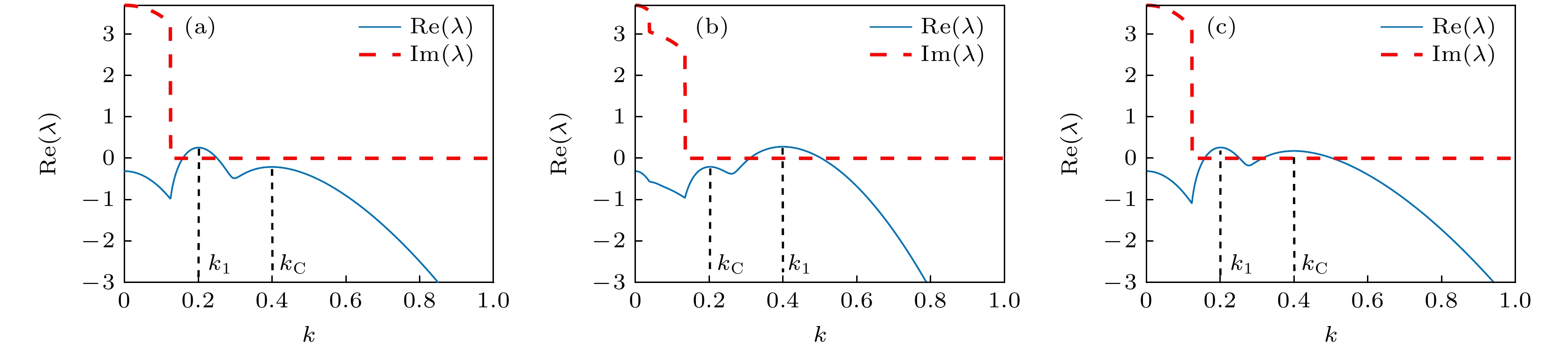
图 1 不同图灵模类型的双层耦合系统的色散关系图 (a) 类型I (
Du1=50 ,Dv1=127 ,Du2=6.6 ,Dv2=81 ,α=0.1 ); (b) 类型II (Du1=12.5 ,Dv1=32 ,Du2=26.5 ,Dv2=320 ,α=0.1 ); (c) 类型III (Du1=50 ,Dv1=127 ,Du2=5.5 ,Dv2=98 ,α=0.1 )Figure 1. Dispersion curves of two-layer coupled systems with different Turing mode types: (a) Type I (
Du1=50 ,Dv1=127 ,Du2=6.6 ,Dv2=81 ,α=0.1 ); (b) type II (Du1=12.5 ,Dv1=32 ,Du2=26.5 ,Dv2=320 ,α=0.1 ); (c) type III (Du1=50 ,Dv1=127 ,Du2=5.5 ,Dv2=98 ,α=0.1 ).
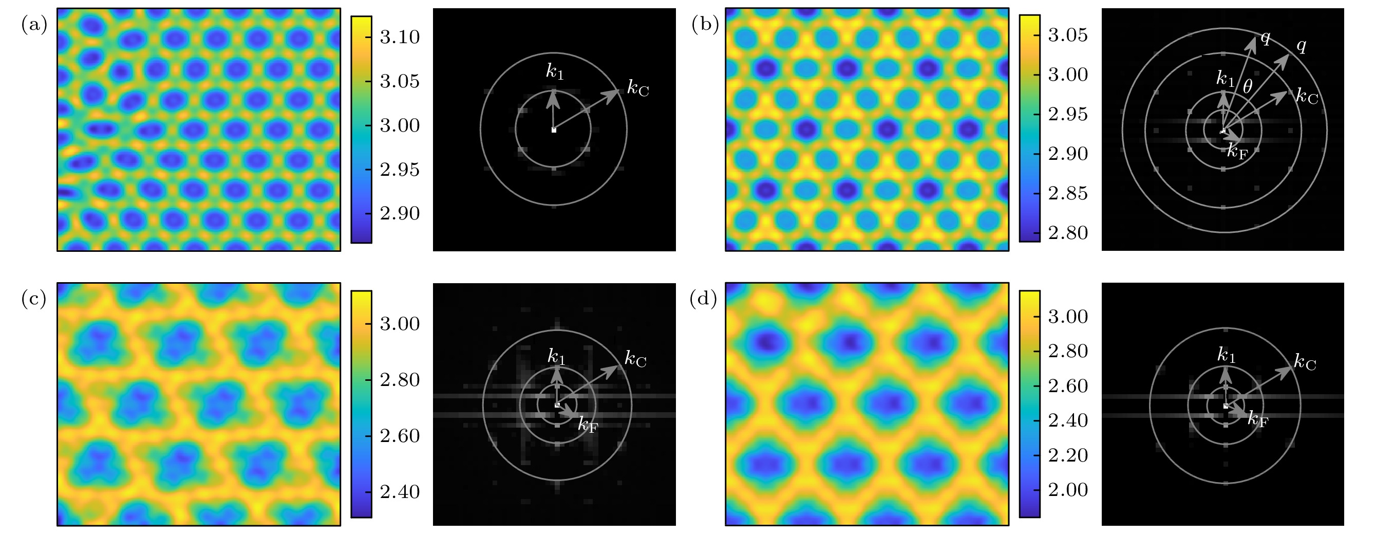
图 2 类型I下不同驱动强度的图灵斑图及其傅里叶频谱图 (a) 超六边形斑图,
w0=0 ; (b) 雪花斑图I,w0=0.1 ; (c) 菱形网格斑图I,w0=0.5 ; (d) 菱形网格斑图II,w0=1.0 (超临界图灵模k1=0.2 , 次临界本征模kC=0.4 , 驱动的波数kF=0.1 ;N=256 ,Δx=Δy=1 )Figure 2. Patterns and Fourier spectrum with different forcing intensity in type I: (a) Super-hexagon pattern,
w0=0 ; (b) snowflake pattern I,w0=0.1 ; (c) rhombus mash pattern I,w0=0.5 ; (d) rhombus mash pattern II,w0=1.0 (Supercritical Turing modek1=0.2 , subcritical eigenmodekC=0.4 , wavenumber of forcingkF=0.1 ;N=256 ,Δx=Δy=1 )
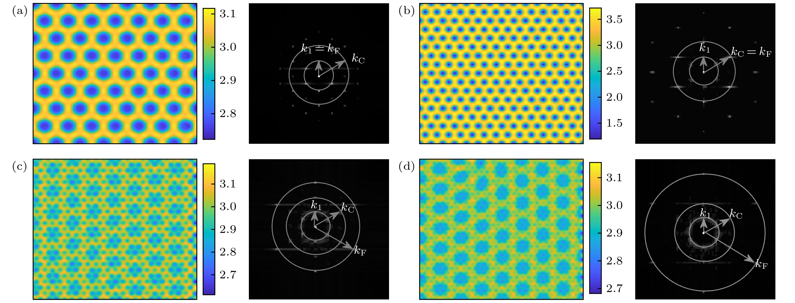
图 3 类型I下不同驱动波数的斑图及其傅里叶频谱图 (a) 超六边形斑图,
kF=0.2 ; (b) 简单六边形蜂窝斑图,kF=0.4 ; (c) 六边形网格斑图I,kF=0.6 ; (d) 六边形网格斑图II,kF=0.8 (超临界图灵模k1=0.2 , 次临界本征模kC=0.4 , 驱动的强度恒为w0=0.1 ,N=256 ,Δx=Δy=1 )Figure 3. Patterns and Fourier spectrum with different forcing wavenumber in type I: (a) Super-hexagon pattern,
kF=0.2 ; (b) simple hexagonal honeycomb pattern,kF=0.4 ; (c) hexagonal mash pattern I,kF=0.6 ; (d) hexagonal mash pattern II,kF=0.8 (Supercritical Turing modek1=0.2 , subcritical eigenmodekC=0.4 , forcing intensityw0=0.1 ,N=256 ,Δx=Δy=1 )
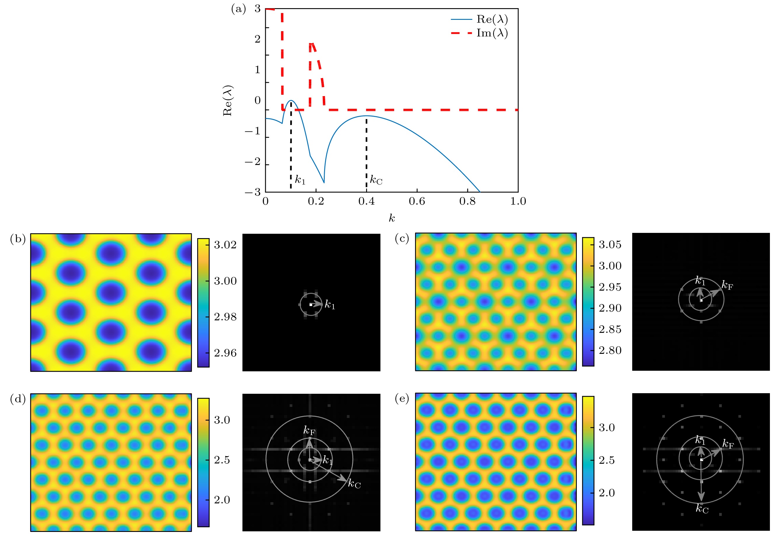
图 4 波数反转后不同驱动强度下的斑图及其傅里叶频谱图 (a) 色散关系图(
k1:kC=1:4 ,Du1=195 ,Dv1=510 ,Du2=6.6 ,Dv2=81 ,α=0.1 ); (b) 简单六边形蜂窝斑图,w0=0 ; (c) 雪花斑图II,w0=0.1 ; (d) 简单六边形蜂窝斑图,w0=0.6 ; (e) 六边形白眼斑图,w0=1.0 (驱动的波数kF=0.2 ;N=256 ,Δx=Δy=1 )Figure 4. Patterns and Fourier spectrum of different forcing intensity after wavenumber inversion: (a) Dispersion curve (
k1:kC= 1:4 ,Du1=195 ,Dv1=510 ,Du2=6.6 ,Dv2=81 ,α=0.1 ); (b) simple hexagonal honeycomb pattern,w0=0 ; (c) snowflake pattern II,w0=0.1 ; (d) simple hexagonal honeycomb pattern,w0=0.6 ; (e) hexagonal white-eye pattern,w0=1.0 (Wavenumber of forcingkF=0.2 ,N=256 ,Δx=Δy=1 )
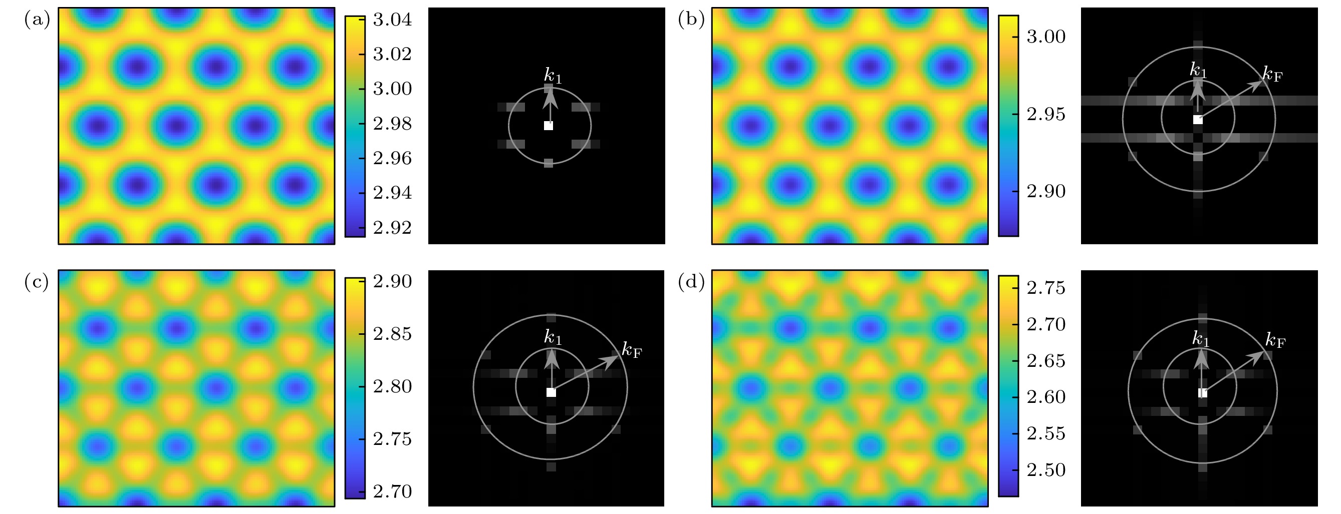
图 5 类型II下不同短波驱动强度的斑图及其傅里叶频谱图 (a) 简单六边形蜂窝斑图,
w0=0 ; (b) 简单六边形蜂窝斑图,w0=0.1 ; (c) 六边形花瓣斑图I,w0=0.5 ; (d) 六边形花瓣斑图II,w0=1.0 (超临界图灵模k1=0.4 , 次临界本征模kC=0.2 , 驱动的波数kF=0.8 ,N=128 ,Δx=Δy=0.5 )Figure 5. Patterns and Fourier spectrum of different short-wave forcing intensity in type II: (a) Simple hexagonal honeycomb pattern,
w0=0 ; (b) simple hexagonal honeycomb pattern,w0=0.1 ; (c) hexagonal petal pattern pattern I,w0=0.5 ; (d) hexagonal petal pattern pattern II;w0=1.0 (Supercritical Turing modek1=0.4 , subcritical eigenmodekC=0.2 , wavenumber of forcingkF=0.8 ,N=128 ,Δx=Δy=0.5 )图 6 类型II下不同长波驱动强度的斑图及其傅里叶频谱图 (a) 简单六边形蜂窝斑图,
w0=0 ; (b) 简单六边形蜂窝斑图,w0=0.1 ; (c) 六边形蜂窝斑图,w0=0.6 ; (d) 黑眼六边形蜂窝斑图,w0=1.0 (超临界图灵模k1=0.4 , 次临界本征模kC=0.2 , 驱动的波数kF=0.1 ,N=256 ,Δx=Δy=1 )Figure 6. Patterns and Fourier spectrum of different long-wave forcing intensity in type II: (a) Simple hexagonal honeycomb pattern,
w0=0 ; (b) simple hexagonal honeycomb pattern,w0=0.1 ; (c) hexagonal honeycomb pattern,w0=0.6 ; (d) black-eye hexagonal honeycomb pattern,w0=1.0 (Supercritical Turing modek1=0.4 , subcritical eigenmodekC=0.2 , wavenumber of forcingkF=0.1 ,N=256 ,Δx=Δy=1 )
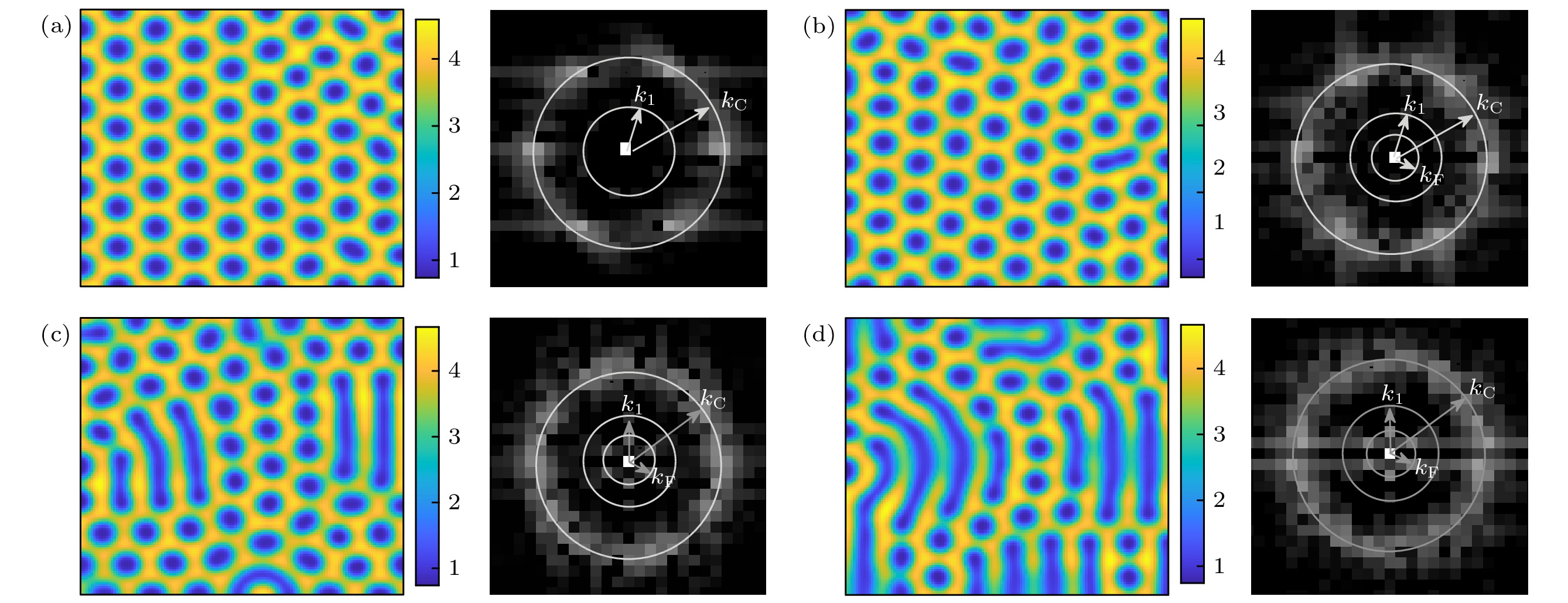
图 7 类型III下不同驱动强度的斑图及其傅里叶频谱图 (a) 简单六边形蜂窝斑图,
w0=0 ; (b) 简单六边形蜂窝斑图,w0=0.1 ; (c) 调制蜂窝斑图,w0=0.5 ; (d) 条纹与蜂窝六边形共存斑图,w0=1.0 (超临界图灵模k1=0.2 , 超临界图灵模kC=0.4 , 驱动的波数kF=0.1 ;N=128 ,Δx=Δy=1 )Figure 7. Patterns and Fourier spectrum with different forcing intensity in type III: (a) Simple hexagonal honeycomb pattern,
w0=0 ; (b) simple hexagonal honeycomb pattern,w0=0.1 ; (c) modulated honeycomb pattern,w0=0.5 ; (d) coexistence of stripe and honeycomb hexagon,w0=1.0 (Supercritical Turing modek1=0.2 , supercritical Turing modekC=0.4 , wavenumber of forcingkF=0.1 ,N=128 ,Δx=Δy=1 )
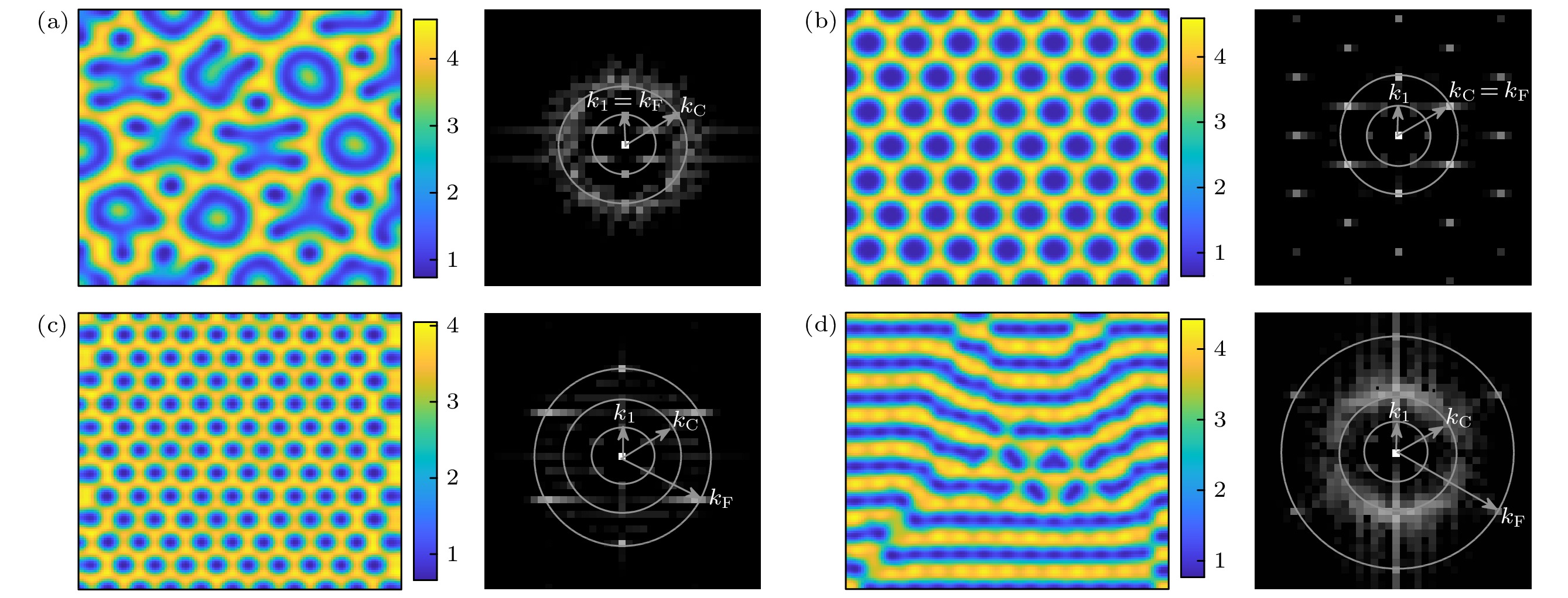
图 8 类型III下不同驱动波数的斑图及其傅里叶频谱图 (a) 复杂斑图,
kF=0.2 ; (b) 简单六边形蜂窝斑图,kF=0.4 ; (c) 简单六边形蜂窝斑图,kF=0.6 ; (d) 条纹斑图,kF=0.8 (超临界图灵模k1=0.2 , 超临界图灵模kC=0.4 , 驱动的强度固定为w0=1.0 ,N=128 ,Δx=Δy=1 )Figure 8. Patterns and Fourier spectrum with different forcing wavenumber in type III: (a) Complex pattern,
kF=0.2 ; (b) simple hexagonal honeycomb pattern,kF=0.4 ; (c) simple hexagonal honeycomb pattern,kF=0.6 ; (d) stripe pattern,kF=0.8 (Supercritical Turing modek1=0.2 , supercritical Turing modekC=0.4 , forcing intensityw0=1.0 ,N=128 ,Δx=Δy=1 ) -
[1] Yochelis A, Gilad E, Nishiura Y, Silber M, Uecker H 2021 Physica D 415 132769
Google Scholar
[2] Sam E M, Hayase Y, Auernhammer G, Vollmer D 2011 Phys. Chem. Chem. Phys. 13 13333
Google Scholar
[3] Perinet N, Juric D, Tuckerman L S 2012 Phys. Rev. Lett. 109 164501
Google Scholar
[4] Alarcón H, Muñoz M H, Perinet N, Mujica N, Gutierrez P, Gordillo L 2020 Phys. Rev. Lett. 125 254505
Google Scholar
[5] Foster J E, Kovach Y E, Lai J, Garcia M C 2020 Plasma Sources Sci. T. 29 034004
Google Scholar
[6] Brauns F, Weyer H, Halatek J, Yoon J, Frey E 2021 Phys. Rev. Lett. 126 104101
Google Scholar
[7] Turing A M 1952 Phil. Trans. R. Soc. B 237 37
Google Scholar
[8] Fuseya Y, Katsuno H, Behnia K, Kapitulnik A 2021 Nat. Phys. 17 1031
Google Scholar
[9] Haas P A, Goldstein R E 2021 Phys. Rev. Lett. 126 238101
Google Scholar
[10] Mau Y, Hagberg A, Meron E 2012 Phys. Rev. Lett. 109 034102
Google Scholar
[11] Mau Y, Haim L, Hagberg A, Meron E 2013 Phys. Rev. E. 88 032917
Google Scholar
[12] Manor R, Hagberg A, Meron E 2009 New J. Phys. 11 063016
Google Scholar
[13] Dolnik M, Berenstein I, Zhabotinsky A M, Epstein I R 2001 Phys. Rev. Lett. 87 238301
Google Scholar
[14] Berenstein I, Yang L F, Dolnik M, Zhabotinsky A M, Epstein I R 2003 Phys. Rev. Lett. 91 058302
Google Scholar
[15] Dolnik M, Jr. Bánsági T, Ansari S, Valent I, Epstein I. R 2011 Phys. Chem. Chem. Phys. 13 12578
Google Scholar
[16] Berenstein I, Yang L F, Dolnik M, Zhabotinsky A M, Epstein I R 2005 J. Phys. Chem. A 109 5382
Google Scholar
[17] Nagao R, Epstein I R, Dolnik. M 2013 J. Phys. Chem. A 117 9120
Google Scholar
[18] Haim L, Hagberg A, Meron E 2015 Chaos 25 064307
Google Scholar
[19] Liu S, Yao C G, Wang X F, Zhao Q 2017 Physica A 467 184
Google Scholar
[20] Berenstein I, Munuzuri A P, Yang L F, Dolnik M, Zhabotinsk A M, Epstein I R 2008 Phys. Rev. E 78 025101
Google Scholar
[21] Barrio R A, Varea C, Aragón J L, Maini P K 1999 Bull. Math. Biol. 61 483
Google Scholar
[22] Li J, Wang H L, Ouyang Q 2014 Chaos 24 023115
Google Scholar
[23] Paul S, Pal K, Ray D S 2020 Phys. Rev. E 102 052209
Google Scholar
[24] 李伟恒, 潘飞, 黎维新, 唐国宁 2015 物理学报 64 198201
Google Scholar
Li W H, Pan F, Li W X, Tang G N 2015 Acta Phys. Sin. 64 198201
Google Scholar
[25] Feng F, Yan J, Liu F C, He Y F 2016 Chin. Phys. B 25 104702
Google Scholar
[26] 刘富成, 刘雅慧, 周志向, 郭雪, 董梦菲 2020 物理学报 69 028201
Google Scholar
Liu F C, Liu Y H, Zhou Z X, Guo X, Dong M F 2020 Acta Phys. Sin. 69 028201
Google Scholar
[27] Miguez D G, Dolnik M, Epstein I R, Munuzuri A P 2011 Phys. Rev. E. 84 046210
Google Scholar
[28] 白婧, 关富荣, 唐国宁 2021 物理学报 70 170502
Google Scholar
Bai J, Guan F R, Tang G N 2021 Acta Phys. Sin. 70 170502
Google Scholar
[29] 李倩昀, 白婧, 唐国宁 2021 物理学报 70 098202
Google Scholar
Li Q Y, Bai J, Tang G N 2021 Acta Phys. Sin. 70 098202
Google Scholar
[30] 张秀芳, 马军, 徐莹, 任国栋 2021 物理学报 70 090502
Google Scholar
Zhang X F, Ma J, Xu Y, Ren G D 2021 Acta Phys. Sin. 70 090502
Google Scholar
[31] Wang Q, Ning W J, Dai D, Zhang Y H 2019 Plasma Process. Polym. 17 1900182
Google Scholar
[32] Sinclair J, Walhout M 2012 Phys. Rev. Lett. 108 035005
Google Scholar
[33] Fan W L, Hou X H, Tian M, Gao K Y, He Y F, Yang Y X, Liu Q, Yao J F, Liu F C, Yuan C X 2022 Plasma Sci. Technol. 24 015402
Google Scholar
[34] Fan W L, Sheng Z M, Dang W, Liang Y Q, Gao K Y, Dong L F 2019 Phys. Rev. Appl. 11 064057
Google Scholar
[35] 刘雅慧, 董梦菲, 刘富成, 田淼, 王硕, 范伟丽 2021 物理学报 70 158201
Google Scholar
Liu Y H, Dong M F, Liu F C, Tian M, Wang S, Fan W L 2021 Acta Phys. Sin. 70 158201
Google Scholar
[36] Fan W L, Liu C Y, Gao K Y, Liang Y Q, Liu F C 2021 Phys. Lett. A 396 127223
Google Scholar
[37] 白占国, 刘富成, 董丽芳 2015 物理学报 64 210505
Google Scholar
Bai Z G, Liu F C, Dong L F 2015 Acta Phys. Sin. 64 210505
Google Scholar
[38] Yang L F, Dolnik M, Zhabotinsky A M, Epstein I R 2002 Phys. Rev. Lett. 88 208303
Google Scholar
Catalog
Metrics
- Abstract views: 5014
- PDF Downloads: 74