光电流驱动下非线性神经元电路的放电模式控制

谢盈; 朱志刚; 张晓锋; 任国栋

doi:10.7498/aps.70.20210676

摘要

放电模态是可以识别生物神经元的电活动, 即细胞内和细胞外的离子被泵送并在细胞内交换的过程. 通过适当的物理刺激, 人工神经元电路可以被设计以重现类似生物神经元的放电模式. 光电管中产生的光电流可以作为信号源, 对神经元电路进行刺激. 但由于不同支路上的通道电流对功能神经元动力学的控制程度不同, 所以光电管接入不同的支路, 将会使神经元电路的放电模式产生很大差异. 本文所采用的非线性神经元是由一个电容器、感应线圈、非线性电阻、两个理想电阻和一个周期电压源组成的FHN (FitzHugh-Nagumo neuron)电路. 在此基础上, 将光电管引入不同的支路来改变通道电流, 以研究光电流的生物物理作用. 当光电管连接到电容上, 光电管被激活从而改变通道电流时, 细胞膜电位可以直接改变, 并切换激发模式. 当光电管串联连接到感应线圈时, 通过感应线圈的感应电流被调节以平衡外部刺激. 这些结果表明, 在本文构建的两类光敏神经元模型中, 相比光电流驱动电感支路, 光电流驱动电容器支路可以更有效地调节膜电位, 大大提高感光灵敏度.

关键词:

Abstract

Firing patterns discern the electrical activities in biological neurons when intracellular and extracellular ions are pumped into cells and exchanged there. Artificial neural circuits can be tamed to reproduce similar firing modes from biological neurons by applying appropriate physical stimuli. Photocurrent generated in the phototube can be used as a signal source, which can stimulate the neural circuits, while the involvement of which branch circuit will be much different because the channel current can control the dynamics of functional neuron to a different degree. In this paper, based on a nonlinear (FitzHugh-Nagumo, FHN) neural circuit composed of one capacitor, induction coil, nonlinear resistor, two ideal resistors and one periodical stimulus, the phototube is incorporated into different branch circuits for changing the channel current and the biophysical role of photocurrent is investigated. The dynamical equations of three types of system are unified, though they fall in different areas in parameter space. The membrane potential can be directly changed and firing modes are switched when photocurrent is activated to change the channel current by connecting the phototube to the capacitor. The induced current across the induction coil is regulated to balance the external stimulus when the phototube is connected to the induction coil in series. The two types of photosensitive neuron models constructed in this paper are compared with the photocurrent driven inductive branch showing that the photocurrent driven capacitive branch can very effectively regulate the membrane potential and greatly improve the photosensitive sensitivity.

Keywords:

作者及机构信息

兰州理工大学物理系, 兰州　730050

通信作者: 朱志刚, zhuzg@lut.edu.cn

基金项目: 国家自然科学基金(批准号: 12072139)和兰州理工大学博士启动经费(批准号: 061906)资助的课题.

Authors and contacts

Department of Physics, Lanzhou University of Technology, Lanzhou 730050, China

Corresponding author: Zhu Zhi-Gang, zhuzg@lut.edu.cn

Funds: Project supported by the National Natural Science Foundation of China (Grant No. 12072139) and the Lanzhou University Technology Doctoral Research Initiation Project, China (Grant No. 061906).

文章全文 : translate this paragraph

参考文献

[1]	Torres J J, Elices I, Marro J 2015 Plos One 10 E0121156 Google Scholar
[2]	Belykh I, De Lange E, Hasler M 2005 Phys. Rev. Lett. 94 188101 Google Scholar
[3]	Wig G S, Schlaggar B L, Petersen S E 2011 Ann. Ny. Acad. Sci. 1224 126 Google Scholar
[4]	Izhikevich E M 2004 IEEE T. Neural. Networ. 15 1063 Google Scholar
[5]	Ozer M, Ekmekci N H 2005 Phys. Lett. A 338 150 Google Scholar
[6]	Bao B C, Liu Z, Xu J P 2010 Electron Lett. 46 237 Google Scholar
[7]	Li Q, Zeng H, Li J 2015 Nonlinear Dynam. 79 2295 Google Scholar
[8]	Song X, Wang C, Ma J, Tang J 2015 Sci. China Technol. Sci. 58 1007 Google Scholar
[9]	Lin W, Wang Y, Ying H, Lai Y C, Wang X 2015 Phys. Rev. E 92 012912 Google Scholar
[10]	Ren G, Tang J, Ma J, Xu Y 2015 Commun. Nonlinear Sci. 29 170 Google Scholar
[11]	Perc M, Marhl M 2005 Phys. Rev. E 71 026229 Google Scholar
[12]	Perc M 2007 Chaos Soliton Fract. 32 1118 Google Scholar
[13]	Takembo C N, Fouda H P E 2020 Sci. Rep. 10 1 Google Scholar
[14]	Sharp A A, O'neil M B, Abbott L, Marder E 1993 Trends Neurosci. 16 389 Google Scholar
[15]	Ma J, Zhang G, Hayat T, Ren G 2019 Nonlinear Dynam. 95 1585 Google Scholar
[16]	Rocha R, Ruthiramoorthy J, Kathamuthu T 2017 Nonlinear Dynam. 88 2577 Google Scholar
[17]	Binczak S, Jacquir S, Bilbault J-M, Kazantsev V B, Nekorkin V I 2006 Neural Networks 19 684 Google Scholar
[18]	Cosp J, Binczak S, Madrenas J, Fernández D 2008 IEEE International Symposium On Circuits And Systems Seattle, WA, USA, May18–21, 2008 pp2370−2373
[19]	Wang C, Chu R, Ma J 2015 Complexity 21 370 Google Scholar
[20]	Volos C, Akgul A, Pham V T, Stouboulos I, Kyprianidis I 2017 Nonlinear Dynam. 89 1047 Google Scholar
[21]	Ma J, Yang Z Q, Yang L J, Tang J 2019 J Zhejiang Univ. Sci A 20 639 Google Scholar
[22]	Karthikeyan A, Cimen M E, Akgul A, Boz A F, Rajagopal K 2021 Nonlinear Dynam. 103 1979 Google Scholar
[23]	Zhang S, Zheng J, Wang X, Zeng Z 2021 Chaos 31 011101 Google Scholar
[24]	Sahin M, Taskiran Z C, Guler H, Hamamci S 2019 Sensor Actuat A 290 107 Google Scholar
[25]	Ren G, Zhou P, Ma J, Cai N, Alsaedi A, Ahmad B 2017 Int. J. Bifurcat Chaos 27 1750187 Google Scholar
[26]	Wang C, Liu Z, Hobiny A, Xu W, Ma J 2020 Chaos Soliton Fract. 134 109697 Google Scholar
[27]	Hindmarsh J L, Rose R 1984 Proc. Roy. Soc. Lond. B: Bio. Sci. 221 87 Google Scholar
[28]	Cao H, Wu Y 2013 Int. J. Bifurcat Chaos 23 1330041 Google Scholar
[29]	Tanaka G, Ibarz B, Sanjuan M A, Aihara K 2006 Chaos 16 013113 Google Scholar
[30]	Zhang J, Huang S, Pang S, Wang M, Gao S 2016 Nonlinear Dynam. 84 1303 Google Scholar
[31]	Usha K, Subha P 2019 Chin. Phys. B 28 020502 Google Scholar
[32]	Wang Q, Lu Q, Chen G, Duan L 2009 Chaos Soliton Fract. 39 918 Google Scholar
[33]	Ma J, Tang J 2015 Sci. China Technol. Sci. 58 2038 Google Scholar
[34]	Lv M, Wang C, Ren G, Ma J, Song X 2016 Nonlinear Dynam. 85 1479 Google Scholar
[35]	Zou W, Senthilkumar D, Zhan M, Kurths J 2013 Phys. Rev. Lett. 111 014101 Google Scholar
[36]	Kenett D Y, Perc M, Boccaletti S 2015 Chaos Soliton Fract. 80 1 Google Scholar
[37]	Ducci S, Treps N, Maître A, Fabre C 2001 Phys. Rev. A 64 023803 Google Scholar
[38]	Wong S T, Plettner T, Vodopyanov K L, Urbanek K, Digonnet M, Byer R L 2008 Opt. Lett. 33 1896 Google Scholar
[39]	Zhang Y, Zhou P, Tang J, Ma J 2021 Chin. J. Phys. 71 72 Google Scholar
[40]	Xu Y, Guo Y, Ren G, Ma J 2020 Appl. Math. Comput. 385 125427 Google Scholar
[41]	Gerasimova S, Gelikonov G, Pisarchik A, Kazantsev V 2015 J. Commun. Technol. 60 900 Google Scholar
[42]	Liu Y, Xu Y, Ma J 2020 Commun Nonlinear Sci. 89 105297 Google Scholar
[43]	Guo Y, Zhu Z, Wang C, Ren G 2020 Optik 218 16499
[44]	Shilnikov A 2012 Nonlinear Dynam. 68 305 Google Scholar
[45]	Duan L, Lu Q, Wang Q 2008 Neurocomputing 72 341 Google Scholar
[46]	Karaoğlu E, Yılmaz E, Merdan H 2016 Neurocomputing 182 102 Google Scholar
[47]	Liu Y, Xu W J, Ma J, Alzahrani F, Hobiny A 2020 Front Inform. Tech. El. 21 1387 Google Scholar

施引文献

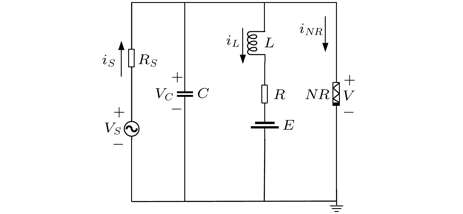
图 1 余弦电压源驱动的简单FHN电路的示意图, 其中NR为非线性电阻, C为电容, L为感应线圈, R和R_S为线性电阻(分压电阻), E为恒压源, V_S为余弦电压源.

Fig. 1. Schematic diagram for the FHN neural circuit. NR is a nonlinear resistor, C is capacitor, L represents induction coil, R andR_S are linear resistors, E is a constant voltage source, and V_S is the external voltage source.

下载: 全尺寸图片幻灯片

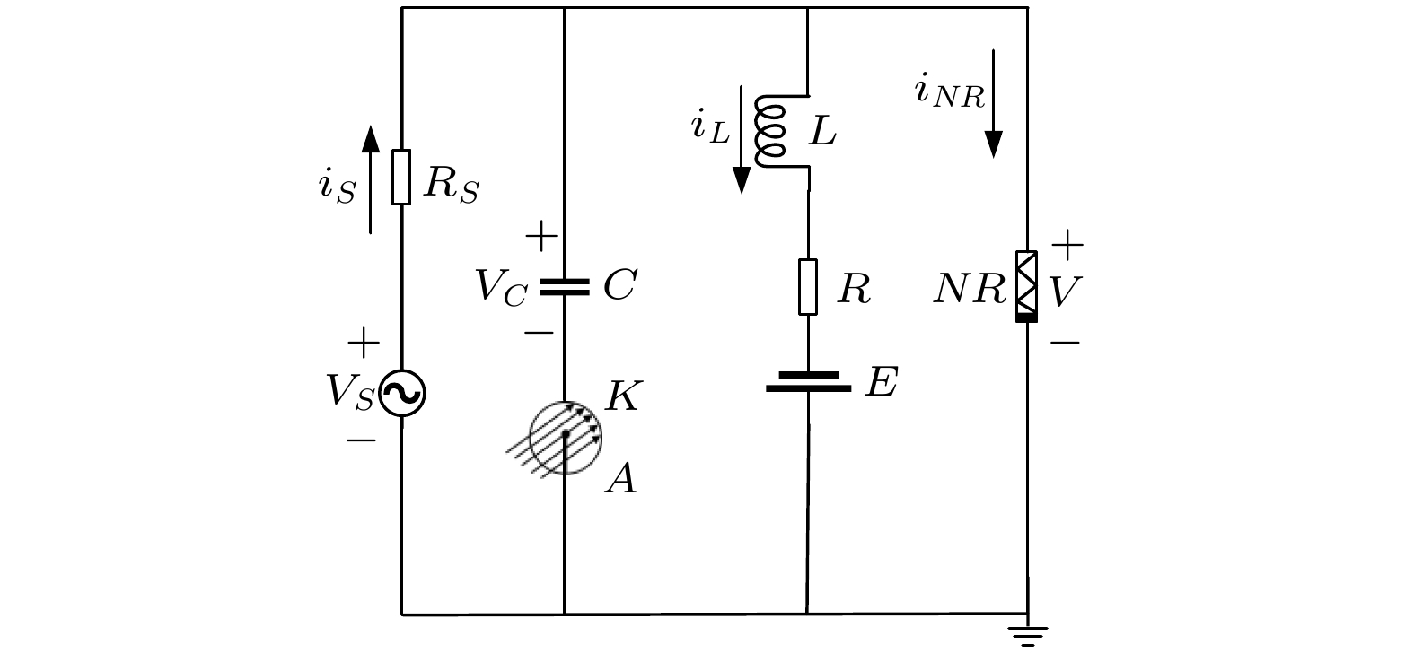
图 2 将光电管和电容串联的FHN电路原理示意图, 其中K表示光电管中的阴极, A表示光电管中的阳极

Fig. 2. Schematic diagram for the FHN neural circuit while phototube couples with capacitor. K denotes cathode and A represents anode in the phototube.

下载: 全尺寸图片幻灯片

图 3 光电管电压与光电流关系图

Fig. 3. Plot of the relationship between voltage and photocurrent.

下载: 全尺寸图片幻灯片

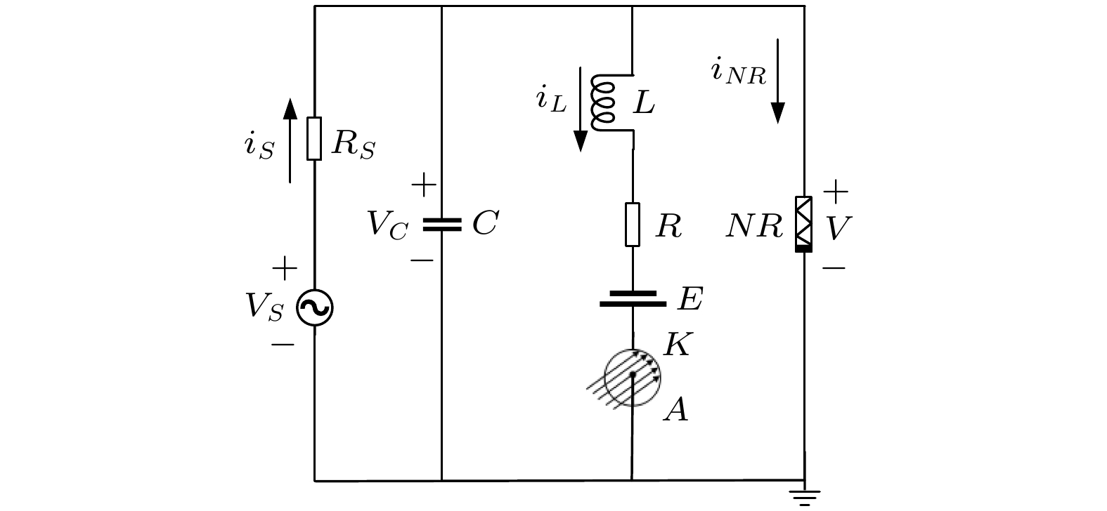
图 4 将光电管和恒压源串联的FHN电路原理示意图

Fig. 4. Schematic diagram for the FHN neural circuit while phototube couples with induction coil.

下载: 全尺寸图片幻灯片

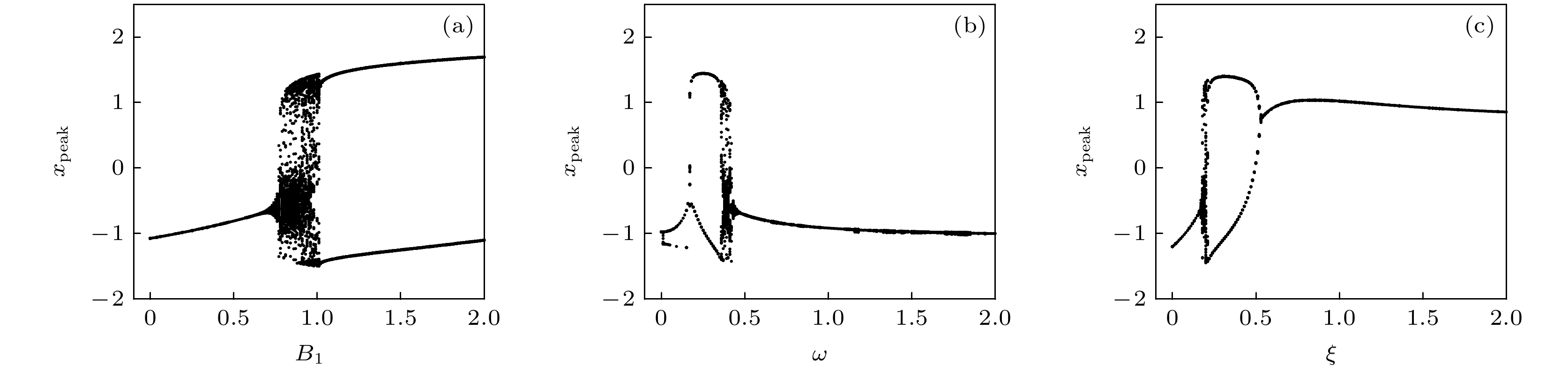
图 5 不同分岔参数(B₁, ω, ξ)下的分岔图　(a) ω = 0.4, ξ = 0.175; (b) B₁ = 0.8, ξ = 0.175; (c) B₁ = 0.8, ω = 0.4, 其中参数a = 0.7, b = 0.8, c = 0.1, 初始值为(x, y) = (0.2, 0.1).

Fig. 5. Bifurcation diagram calculated by changing the bifurcation parameters (B, ω, ξ) at a = 0.7, b = 0.8, c = 0.1, initial parameters (x, y) = (0.2, 0.1): (a) ω = 0.4, ξ = 0.175; (b) B₁ = 0.8, ξ = 0.175; (c) B₁ = 0.8, ω = 0.4.

下载: 全尺寸图片幻灯片

图 6 不同分岔参数(B₁, ω, ξ)下的李雅普诺夫指数图　(a) ω = 0.4, ξ = 0.175; (b) B₁ = 0.8, ξ = 0.175; (c) B₁ = 0.8, ω = 0.4, 其中参数a = 0.7, b = 0.8, c = 0.1, 初始值为(x, y) = (0.2, 0.1).

Fig. 6. Distribution for the Lyapunov exponent spectrum calculated by changing the bifurcation parameters (B₁, ω, ξ) at a = 0.7, b = 0.8, c = 0.1, initial parameters (x, y) = (0.2, 0.1): (a) ω = 0.4, ξ = 0.175; (b) B₁ = 0.8, ξ = 0.175; (c) B₁ = 0.8, ω = 0.4.

下载: 全尺寸图片幻灯片

图 7 不同分岔参数下的时间序列图, 其中固定参数ω = 0.4, ξ = 0.175, (a1) B₁ = 0.001, (a2) B₁ = 0.5, (a3) B₁ = 0.9, (a4) B₁ = 1.1; 固定参数B₁ = 0.8, ξ = 0.175时, (b1) ω = 0.11, (b2) ω = 0.31, (b3) ω = 0.4, (b4) ω = 0.5; 固定参数B₁ = 0.8, ω = 0.4时, (c1) ξ = 0.15, (c2) ξ = 0.175, (c3) ξ = 0.21, (c4) ξ = 0.45. 参数a = 0.7, b = 0.8, c = 0.1, 初始值为(x, y) = (0.2, 0.1).

Fig. 7. Firing patterns generated by applying different bifurcation parameters at a = 0.7, b = 0.8, c = 0.1, initial parameters (x, y) = (0.2, 0.1): (a1) B₁ = 0.001, (a2) B₁ = 0.5, (a3) B₁ = 0.9, (a4) B₁ = 1.1 with fixed parameters ω = 0.4, ξ = 0.175; (b1) ω = 0.11, (b2) ω = 0.31, (b3) ω = 0.4, (b4) ω = 0.5 with fixed parameters B₁ = 0.8, ξ = 0.175; (c1) ξ = 0.15, (c2) ξ = 0.175, (c3) ξ = 0.21, (c4) ξ = 0.45 with fixed parameters B₁ = 0.8, ω = 0.4.

下载: 全尺寸图片幻灯片

图 8 不同分岔参数ω下, 关于B₂的分岔图　(a) ω = 0.001; (b) ω = 0.01; (c) ω = 0.1; (d) ω = 0.4; 其中参数a = 0.7, b = 0.8, c = 0.1, B₁ = 0.8, ξ = 0.175, 初始值为(x, y) = (0.2, 0.1)

Fig. 8. Bifurcation diagram of B₂ calculated by changing the bifurcation parameter ω at a = 0.7, b = 0.8, c = 0.1, B₁ = 0.8, ξ = 0.175, initial parameters (x, y) = (0.2, 0.1): (a) ω = 0.001; (b) ω = 0.01; (c) ω = 0.1; (d) ω = 0.4.

下载: 全尺寸图片幻灯片

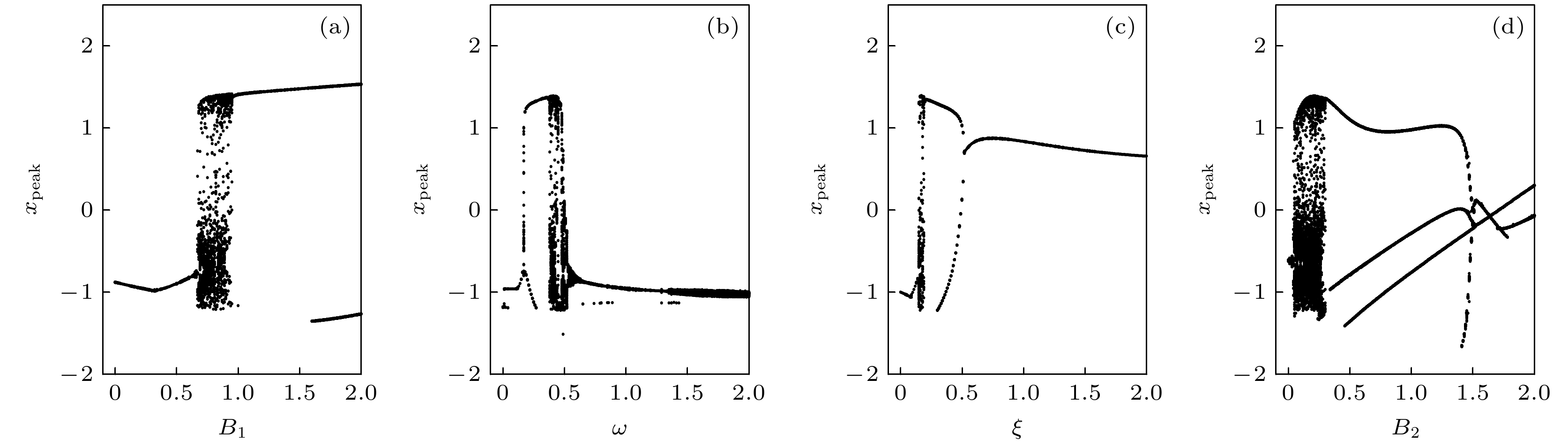
图 9 不同分岔参数(B₁, ω, ξ, B₂)下的分岔图　(a) B₂ = 0.2, ξ = 0.175, ω = 0.4; (b) B₂ = 0.2, B₁ = 0.8, ξ = 0.175; (c) B₂ = 0.2, B₁ = 0.8, ω = 0.4; (d) B₁ = 0.8, ξ = 0.175, ω = 0.4; 其中参数 a = 0.7, b = 0.8, c = 0.1, 初始值为 (x, y) = (0.2, 0.1).

Fig. 9. Bifurcation diagram calculated by changing the bifurcation parameters (B₁, ω, ξ, B₂) at a = 0.7, b = 0.8, c = 0.1, initial parameters (x, y) = (0.2, 0.1): (a) B₂ = 0.2, ξ = 0.175, ω = 0.4; (b) B₂ = 0.2, B₁ = 0.8, ξ = 0.175; (c) B₂ = 0.2, B₁ = 0.8, ω = 0.4; (d) B₁ = 0.8, ξ = 0.175, ω = 0.4.

下载: 全尺寸图片幻灯片

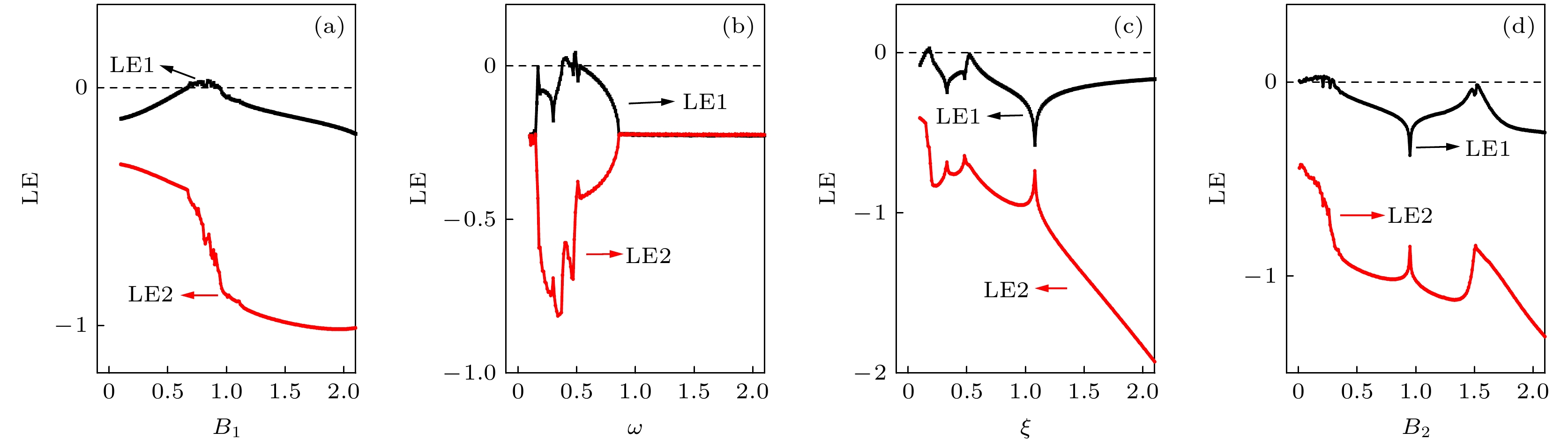
图 10 不同分岔参数(B₁, ω, ξ, B₂)下的李雅普诺夫指数图　(a) B₂ = 0.2, ξ = 0.175, ω = 0.4; (b) B₂ = 0.2, B₁ = 0.8, ξ = 0.175; (c) B₂ = 0.2, B₁ = 0.8, ω = 0.4; (d) B₁ = 0.8, ξ = 0.175, ω = 0.4; 其中参数 a = 0.7, b = 0.8, c = 0.1, 初始值为(x, y) = (0.2, 0.1).

Fig. 10. Distribution for the Lyapunov exponent spectrum calculated by changing the bifurcation parameters (B₁, ω, ξ, B₂) at a = 0.7, b = 0.8, c = 0.1, initial parameters (x, y) = (0.2, 0.1): (a) B₂ = 0.2, ξ = 0.175, ω = 0.4; (b) B₂ = 0.2, B₁ = 0.8, ξ = 0.175; (c) B₂ = 0.2, B₁ = 0.8, ω = 0.4; (d) B₁ = 0.8, ξ = 0.175, ω = 0.4.

下载: 全尺寸图片幻灯片

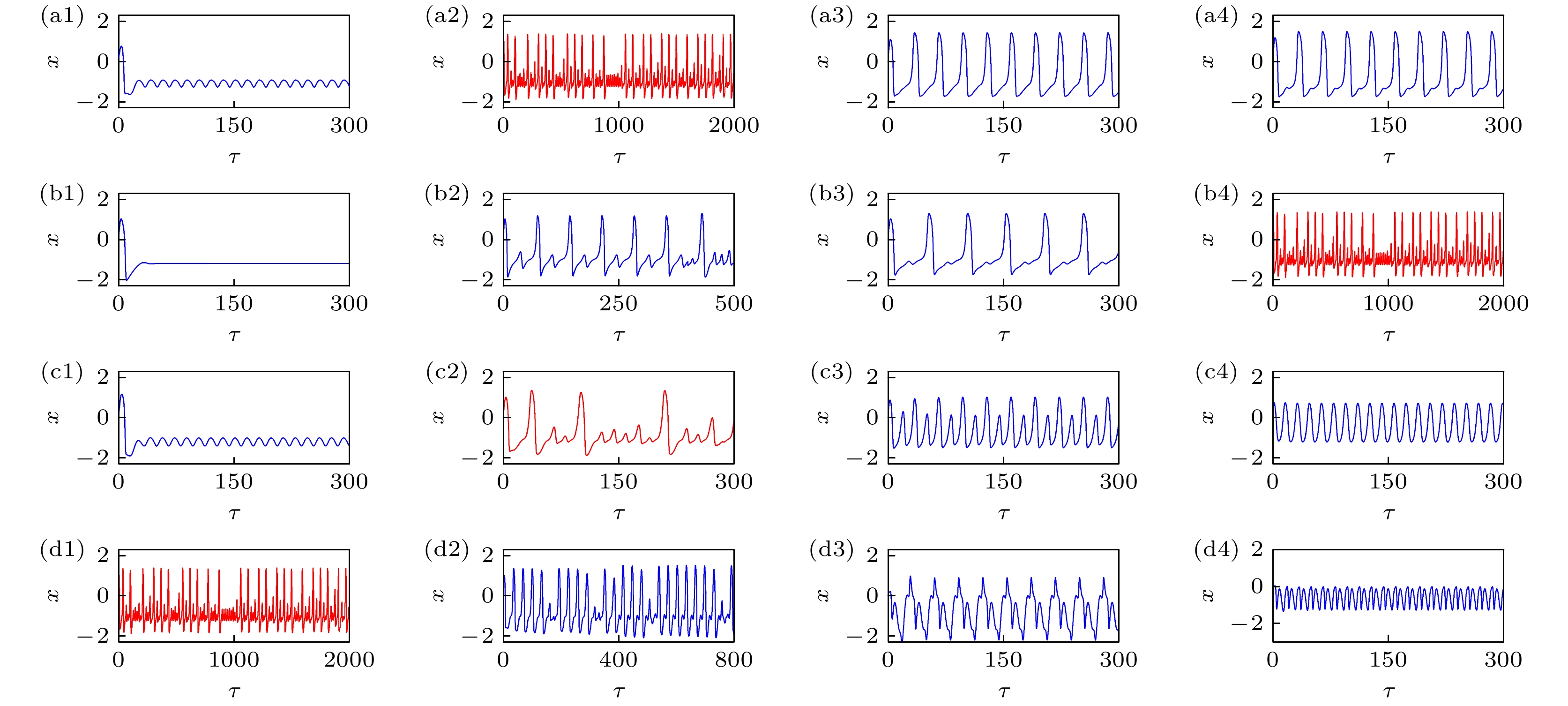
图 11 不同分岔参数下的时间序列图, 其中固定参数ω = 0.4, ξ = 0.175, B₂ = 0.2时, (a1) B₁ = 0.1, (a2) B₁ = 0.8, (a3) B₁ = 1.2, (a4) B₁ = 1.75; 固定参数B₁ = 0.8, ξ = 0.175, B₂ = 0.2时, (b1) ω = 0.001, (b2) ω = 0.18, (b3) ω = 0.25, (b4) ω = 0.4; 固定参数B₁ = 0.8, ω = 0.4, B₂ = 0.2时, (c1) ξ = 0.005, (c2) ξ = 0.175, (c3) ξ = 0.5, (c4) ξ = 1.5; 固定参数B₁ = 0.8, ω = 0.4, ξ = 0.175时, (d1) B₂ = 0.2, (d2) B₂ = 0.28, (d3) B₂ = 1.0, (d4) B₂ = 1.6. 其中参数a = 0.7, b = 0.8, c = 0.1, 初始值为(x, y) = (0.2, 0.1).

Fig. 11. Firing patterns generated by applying different bifurcation parameters at a = 0.7, b = 0.8, c = 0.1, initial parameters (x, y) = (0.2, 0.1): (a1) B₁ = 0.1, (a2) B₁ = 0.8, (a3) B₁ = 1.2, (a4) B₁ = 1.75 with fixed parameters ω = 0.4, ξ = 0.175, B₂ = 0.2; (b1) ω = 0.001, (b2) ω = 0.18, (b3) ω = 0.25, (b4) ω = 0.4 with fixed parameters B₁ = 0.8, ξ = 0.175, B₂ = 0.2; (c1) ξ = 0.005, (c2) ξ = 0.175, (c3) ξ = 0.5, (c4) ξ = 1.5 with fixed parameters B₁ = 0.8, ω = 0.4, B₂ = 0.2; (d1) B₂ = 0.2, (d2) B₂ = 0.28, (d3) B₂ = 1.0, (d4) B₂ = 1.6 with fixed parameters B₁ = 0.8, ω = 0.4, ξ = 0.175.

下载: 全尺寸图片幻灯片

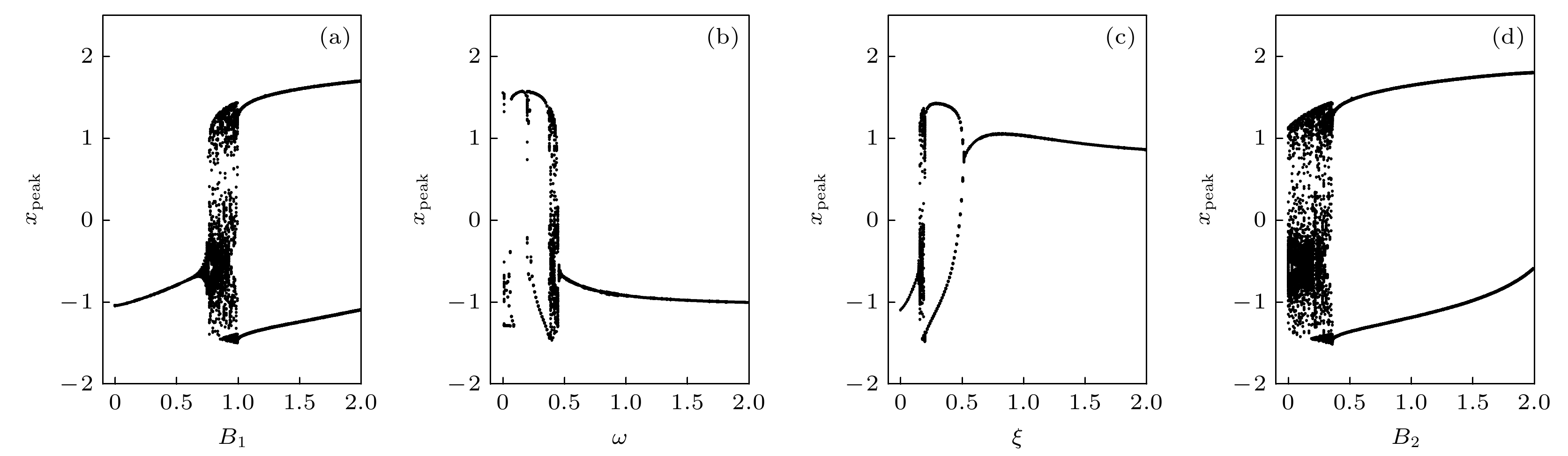
图 12 不同分岔参数(B₁, ω, ξ, B₂)下的分岔图　(a) B₂ = 0.2, ξ = 0.175, ω = 0.4; (b) B₂ = 0.2, B₁ = 0.8, ξ = 0.175; (c) B₂ = 0.2, B₁ = 0.8, ω = 0.4; (d) B₁ = 0.8, ξ = 0.175, ω = 0.4; 其中参数a = 0.7, b = 0.8, c = 0.1, 初始值为(x, y) = (0.2, 0.1)

Fig. 12. Bifurcation diagram calculated by changing the bifurcation parameters (B₁, ω, ξ, B₂) at a = 0.7, b = 0.8, c = 0.1, initial parameters (x, y) = (0.2, 0.1): (a) B₂ = 0.2, ξ = 0.175, ω = 0.4; (b) B₂ = 0.2, B₁ = 0.8, ξ = 0.175; (c) B₂ = 0.2, B₁ = 0.8, ω = 0.4; (d) B₁ = 0.8, ξ = 0.175, ω = 0.4.

下载: 全尺寸图片幻灯片

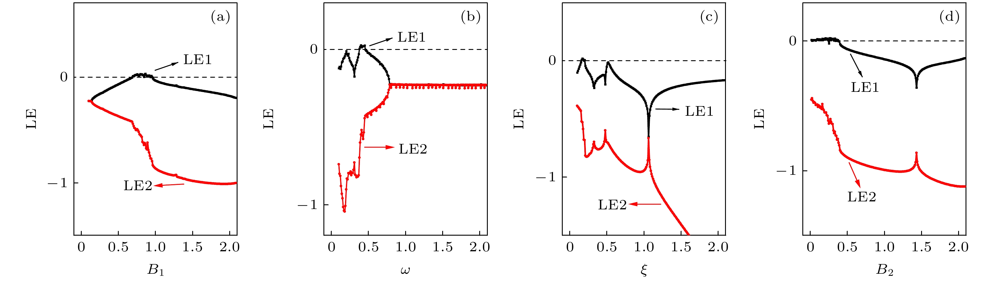
图 13 不同分岔参数(B₁, ω, ξ, B₂)下的李雅普诺夫指数图　(a) B₂ = 0.2, ξ = 0.175, ω = 0.4; (b) B₂ = 0.2, B₁ = 0.8, ξ = 0.175; (c) B₂ = 0.2, B₁ = 0.8, ω = 0.4; (d) B₁ = 0.8, ξ = 0.175, ω = 0.4; 其中参数a = 0.7, b = 0.8, c = 0.1, 初始值为 (x, y) = (0.2, 0.1)

Fig. 13. Lyapunov exponent spectrum calculated by changing the bifurcation parameters (B₁, ω, ξ, B₂) at a = 0.7, b = 0.8, c = 0.1, initial parameters (x, y) = (0.2, 0.1): (a) B₂ = 0.2, ξ = 0.175, ω = 0.4; (b) B₂ = 0.2, B₁ = 0.8, ξ = 0.175; (c) B₂ = 0.2, B₁ = 0.8, ω = 0.4; (d) B₁ = 0.8, ξ = 0.175, ω = 0.4.

下载: 全尺寸图片幻灯片

[1]	Torres J J, Elices I, Marro J 2015 Plos One 10 E0121156 Google Scholar
[2]	Belykh I, De Lange E, Hasler M 2005 Phys. Rev. Lett. 94 188101 Google Scholar
[3]	Wig G S, Schlaggar B L, Petersen S E 2011 Ann. Ny. Acad. Sci. 1224 126 Google Scholar
[4]	Izhikevich E M 2004 IEEE T. Neural. Networ. 15 1063 Google Scholar
[5]	Ozer M, Ekmekci N H 2005 Phys. Lett. A 338 150 Google Scholar
[6]	Bao B C, Liu Z, Xu J P 2010 Electron Lett. 46 237 Google Scholar
[7]	Li Q, Zeng H, Li J 2015 Nonlinear Dynam. 79 2295 Google Scholar
[8]	Song X, Wang C, Ma J, Tang J 2015 Sci. China Technol. Sci. 58 1007 Google Scholar
[9]	Lin W, Wang Y, Ying H, Lai Y C, Wang X 2015 Phys. Rev. E 92 012912 Google Scholar
[10]	Ren G, Tang J, Ma J, Xu Y 2015 Commun. Nonlinear Sci. 29 170 Google Scholar
[11]	Perc M, Marhl M 2005 Phys. Rev. E 71 026229 Google Scholar
[12]	Perc M 2007 Chaos Soliton Fract. 32 1118 Google Scholar
[13]	Takembo C N, Fouda H P E 2020 Sci. Rep. 10 1 Google Scholar
[14]	Sharp A A, O'neil M B, Abbott L, Marder E 1993 Trends Neurosci. 16 389 Google Scholar
[15]	Ma J, Zhang G, Hayat T, Ren G 2019 Nonlinear Dynam. 95 1585 Google Scholar
[16]	Rocha R, Ruthiramoorthy J, Kathamuthu T 2017 Nonlinear Dynam. 88 2577 Google Scholar
[17]	Binczak S, Jacquir S, Bilbault J-M, Kazantsev V B, Nekorkin V I 2006 Neural Networks 19 684 Google Scholar
[18]	Cosp J, Binczak S, Madrenas J, Fernández D 2008 IEEE International Symposium On Circuits And Systems Seattle, WA, USA, May18–21, 2008 pp2370−2373
[19]	Wang C, Chu R, Ma J 2015 Complexity 21 370 Google Scholar
[20]	Volos C, Akgul A, Pham V T, Stouboulos I, Kyprianidis I 2017 Nonlinear Dynam. 89 1047 Google Scholar
[21]	Ma J, Yang Z Q, Yang L J, Tang J 2019 J Zhejiang Univ. Sci A 20 639 Google Scholar
[22]	Karthikeyan A, Cimen M E, Akgul A, Boz A F, Rajagopal K 2021 Nonlinear Dynam. 103 1979 Google Scholar
[23]	Zhang S, Zheng J, Wang X, Zeng Z 2021 Chaos 31 011101 Google Scholar
[24]	Sahin M, Taskiran Z C, Guler H, Hamamci S 2019 Sensor Actuat A 290 107 Google Scholar
[25]	Ren G, Zhou P, Ma J, Cai N, Alsaedi A, Ahmad B 2017 Int. J. Bifurcat Chaos 27 1750187 Google Scholar
[26]	Wang C, Liu Z, Hobiny A, Xu W, Ma J 2020 Chaos Soliton Fract. 134 109697 Google Scholar
[27]	Hindmarsh J L, Rose R 1984 Proc. Roy. Soc. Lond. B: Bio. Sci. 221 87 Google Scholar
[28]	Cao H, Wu Y 2013 Int. J. Bifurcat Chaos 23 1330041 Google Scholar
[29]	Tanaka G, Ibarz B, Sanjuan M A, Aihara K 2006 Chaos 16 013113 Google Scholar
[30]	Zhang J, Huang S, Pang S, Wang M, Gao S 2016 Nonlinear Dynam. 84 1303 Google Scholar
[31]	Usha K, Subha P 2019 Chin. Phys. B 28 020502 Google Scholar
[32]	Wang Q, Lu Q, Chen G, Duan L 2009 Chaos Soliton Fract. 39 918 Google Scholar
[33]	Ma J, Tang J 2015 Sci. China Technol. Sci. 58 2038 Google Scholar
[34]	Lv M, Wang C, Ren G, Ma J, Song X 2016 Nonlinear Dynam. 85 1479 Google Scholar
[35]	Zou W, Senthilkumar D, Zhan M, Kurths J 2013 Phys. Rev. Lett. 111 014101 Google Scholar
[36]	Kenett D Y, Perc M, Boccaletti S 2015 Chaos Soliton Fract. 80 1 Google Scholar
[37]	Ducci S, Treps N, Maître A, Fabre C 2001 Phys. Rev. A 64 023803 Google Scholar
[38]	Wong S T, Plettner T, Vodopyanov K L, Urbanek K, Digonnet M, Byer R L 2008 Opt. Lett. 33 1896 Google Scholar
[39]	Zhang Y, Zhou P, Tang J, Ma J 2021 Chin. J. Phys. 71 72 Google Scholar
[40]	Xu Y, Guo Y, Ren G, Ma J 2020 Appl. Math. Comput. 385 125427 Google Scholar
[41]	Gerasimova S, Gelikonov G, Pisarchik A, Kazantsev V 2015 J. Commun. Technol. 60 900 Google Scholar
[42]	Liu Y, Xu Y, Ma J 2020 Commun Nonlinear Sci. 89 105297 Google Scholar
[43]	Guo Y, Zhu Z, Wang C, Ren G 2020 Optik 218 16499
[44]	Shilnikov A 2012 Nonlinear Dynam. 68 305 Google Scholar
[45]	Duan L, Lu Q, Wang Q 2008 Neurocomputing 72 341 Google Scholar
[46]	Karaoğlu E, Yılmaz E, Merdan H 2016 Neurocomputing 182 102 Google Scholar
[47]	Liu Y, Xu W J, Ma J, Alzahrani F, Hobiny A 2020 Front Inform. Tech. El. 21 1387 Google Scholar

[1]	郭慧朦, 梁燕, 董玉姣, 王光义. 蔡氏结型忆阻器的简化及其神经元电路的硬件实现. 物理学报, 2023, 72(7): 070501. doi: 10.7498/aps.72.20222013
[2]	梁艳美, 陆博, 古华光. 利用双慢变量的快慢变量分离分析新脑皮层神经元Wilson模型的复杂电活动. 物理学报, 2022, 71(23): 230502. doi: 10.7498/aps.71.20221416
[3]	赵雅琪, 刘谋天, 赵勇, 段利霞. 耦合前包钦格复合体神经元中复杂混合簇放电的动力学. 物理学报, 2021, 70(12): 120501. doi: 10.7498/aps.70.20210093
[4]	丁学利, 古华光, 贾冰, 李玉叶. 抑制性自突触诱发耦合Morris-Lecar神经元电活动的超前同步. 物理学报, 2021, 70(21): 218701. doi: 10.7498/aps.70.20210912
[5]	张秀芳, 马军, 徐莹, 任国栋. 光电管耦合FitzHugh-Nagumo神经元的同步. 物理学报, 2021, 70(9): 090502. doi: 10.7498/aps.70.20201953
[6]	华洪涛, 陆博, 古华光. 兴奋性自突触引起神经簇放电频率降低或增加的非线性机制. 物理学报, 2020, 69(9): 090502. doi: 10.7498/aps.69.20191709
[7]	曹奔, 关利南, 古华光. 兴奋性作用诱发神经簇放电个数不增反降的分岔机制. 物理学报, 2018, 67(24): 240502. doi: 10.7498/aps.67.20181675
[8]	任国栋, 武刚, 马军, 陈旸. 一类自突触作用下神经元电路的设计和模拟. 物理学报, 2015, 64(5): 058702. doi: 10.7498/aps.64.058702
[9]	吴旋律, 肖国春, 雷博. 数字控制单相全桥电压型逆变电路的改进离散迭代模型. 物理学报, 2013, 62(5): 050503. doi: 10.7498/aps.62.050503
[10]	冯朝文, 蔡理, 杨晓阔, 康强, 彭卫东, 柏鹏. 单电子晶体管与金属氧化物半导体混合电路构造的一维离散混沌系统研究. 物理学报, 2012, 61(8): 080503. doi: 10.7498/aps.61.080503
[11]	季颖, 毕勤胜. 高维广义蔡氏电路中的快慢动力学行为及其分岔分析. 物理学报, 2012, 61(1): 010202. doi: 10.7498/aps.61.010202
[12]	李群宏, 闫玉龙, 杨丹. 耦合电路系统的分岔研究. 物理学报, 2012, 61(20): 200505. doi: 10.7498/aps.61.200505
[13]	冯朝文, 蔡理, 康强, 彭卫东, 柏鹏, 王甲富. 基于单电子晶体管 - 金属氧化物场效应晶体管电路的离散混沌系统实现. 物理学报, 2011, 60(11): 110502. doi: 10.7498/aps.60.110502
[14]	古华光, 朱洲, 贾冰. 一类新的混沌神经放电的动力学特征的实验和数学模型研究. 物理学报, 2011, 60(10): 100505. doi: 10.7498/aps.60.100505
[15]	陈章耀, 毕勤胜. Jerk系统耦合的分岔和混沌行为. 物理学报, 2010, 59(11): 7669-7678. doi: 10.7498/aps.59.7669
[16]	张晓芳, 陈章耀, 毕勤胜. 非线性电路通向混沌的演化过程. 物理学报, 2010, 59(5): 3057-3065. doi: 10.7498/aps.59.3057
[17]	冯朝文, 蔡理, 张立森, 杨晓阔, 赵晓辉. SETMOS实现多涡卷蔡氏电路的研究. 物理学报, 2010, 59(12): 8426-8431. doi: 10.7498/aps.59.8426
[18]	张晓芳, 陈章耀, 毕勤胜. 耦合电路中的复杂振荡行为分析. 物理学报, 2009, 58(5): 2963-2970. doi: 10.7498/aps.58.2963
[19]	张维, 周淑华, 任勇, 山秀明. Turbo译码算法的分岔与控制. 物理学报, 2006, 55(2): 622-627. doi: 10.7498/aps.55.622
[20]	郝建红, 丁武. 行波管放大器中辐射场的极限环振荡和混沌. 物理学报, 2003, 52(4): 906-910. doi: 10.7498/aps.52.906

计量

文章访问数: 3520
PDF下载量: 87
被引次数: 0

姓名
邮箱
手机号码
标题
留言内容
验证码

搜索

留言板

光电流驱动下非线性神经元电路的放电模式控制