


-
极性分子由于其本身的不对称性, 在强激光场的作用下展现出丰富且复杂的电子动力学现象. 本文利用三维含时Hartree-Fock方法研究了极性分子CO的高次谐波产生过程. 通过高次谐波谱和时频分析结果可知,当激光偏振沿分子轴方向时, 来自C和O两侧的电子对高次谐波的产生具有不同的贡献. 对于平台区较低阶的谐波, 仅C侧电离的电子参与谐波的产生. 而对于较高阶的谐波, C和O两侧的电子共同参与谐波的辐射. 并且, 随着激光偏振与分子轴的夹角θ逐渐增大, C和O两侧电子对谐波强度贡献的差异越来越小. 在高次谐波谱中能量28 eV附近发现了明显的形状共振峰, 随后通过强场近似理论解析了其不对称性. 本文的工作有助于推动高次谐波谱在追踪电子超快动力学和研究极性分子结构方面的应用.
-
关键词:
- 高次谐波 /
- 极性分子 /
- 含时Hartree-Fock /
- 形状共振
Compared with nonpolar molecules, owing to the inherent asymmetry, polar molecules exhibit rich and very complex electronic dynamics under the interaction with strong laser fields. In this work, high-order harmonic generation (HHG) of polar molecules CO is investigated by using the three-dimensional time-dependent Hartree-Fock (3D-TDHF) theory, with all electrons active. Through the high harmonic spectra and time-frequency analyses, it is found that when the laser field polarizes along the molecular axis, the ionized electrons from the two sides (C side and O side) contribute differently to the harmonic radiation. On the one hand, the harmonic intensity from the C side is greater than that from the O side, which is caused by the ionization rate. On the other hand, for the lower-order (7th–17th order) harmonics of plateau region, only the electrons from the C side participate in the HHG. However, for its higher part (18th–36th order), the electrons from both C side and O side contribute to high harmonics simultaneously. Moreover, the difference between contributions from two sides is related to the alignment angle θ between the laser polarization and the molecular axis, and it reaches a maximum value around θ = 0º and a minimum value around θ = 90º. There are two strong resonances around harmonic order H12.6 (19.5 eV) and H18 (27.9 eV) in the harmonic spectra when θ = 0º. The first resonance around H12.6 reveals that part of electrons ionized from the C side recombine to the vicinity of the further O nucleus. Near the second resonance around H18, there appears a shape resonance. Nevertheless, the shape resonances from the C and O sides are disparate. Based on the strong-field approximation theory, the ratio between photoionization cross sections from C and O sides around the shape resonance is calculated. The ratio is about 5.5 from 3D-TDHF, which is greater than the result of 3 simulated by ePloyScat, where only HOMO is considered. This discrepancy reveals that multi-electron effects enhance the asymmetry of polar molecules. This work provides an in-depth insight into the asymmetry in HHG of polar molecules, which benefits the generation of isolated attosecond pulse . It also promotes the application of high harmonic spectra in tracking the ultrafast dynamics of electrons.-
Keywords:
- high-order harmonic generation /
- polar molecule /
- time-dependent Hartree–Fock /
- shape resonance
[1] McPherson A, Gibson G, Jara H, Johann U, Luk T S, McIntyre I A, Boyer K, Rhodes C K 1987 J. Opt. Soc. Am. B: Opt. Phys. 4 595
 Google Scholar
[2] Ferray M, L'Huillier A, Li X F, Lompre L A, Mainfray G, Manus C 1988 J. Phys. B: At. Mol. Opt. Phys. 21 L31
Google Scholar
[3] Brabec T, Krausz F 2000 Rev. Mod. Phys. 72 545
Google Scholar
[4] Krausz F, Ivanov M 2009 Rev. Mod. Phys. 81 163
Google Scholar
[5] Pazourek R, Nagele S, Burgdörfer J 2015 Rev. Mod. Phys. 87 765
Google Scholar
[6] Mourou G 2019 Rev. Mod. Phys. 91 030501
Google Scholar
[7] Krause J L, Schafer K J, Kulander K C 1992 Phys. Rev. Lett. 68 3535
Google Scholar
[8] Corkum P B 1993 Phys. Rev. Lett. 71 1994
Google Scholar
[9] Lewenstein M, Balcou P, Ivanov M Y, L’Huillier A, Corkum P B 1994 Phys. Lett. A 49 2117
Google Scholar
[10] Yang Y, Liu L, Zhao J, Tu Y, Liu J, Zhao Z 2021 J. Phys. B:At. Mol. Opt. Phys. 54 144009
Google Scholar
[11] Huang Y, Zhao J, Shu Z, Zhu Y, Liu J, Dong W, Wang X, Lü Z, Zhang D, Yuan J, Chen J, Zhao Z 2021 Ultrafast Science 2021 9837107
Google Scholar
[12] Li L, Zhang Y, Lan P, Huang T, Zhu X, Zhai C, Yang K, He L, Zhang Q, Cao W, Lu P 2021 Phys. Rev. Lett. 126 187401
Google Scholar
[13] Ghimire S, Reis D A 2019 Nat. Phys. 15 10
Google Scholar
[14] Liu L, Zhao J, Dong W, Liu J, Huang Y, Zhao Z 2017 Phys. Lett. A 96 053403
Google Scholar
[15] Liu L, Zhao J, Yuan J M, Zhao Z X 2019 Chin. Phys. B 28 114205
Google Scholar
[16] Luu T T, Yin Z, Jain A, Gaumnitz T, Pertot Y, Ma J, Wörner H J 2018 Nat. Commun. 9 3723
Google Scholar
[17] Zeng A W, Bian X B 2020 Phys. Rev. Lett. 124 203901
Google Scholar
[18] Hu H, Li N, Liu P, Li R, Xu Z 2017 Phys. Rev. Lett. 119 173201
Google Scholar
[19] Ren Z, Yang Y, Zhu Y, Zan X, Zhao J, Zhao Z 2021 J. Phys. B: At. Mol. Opt. Phys. 54 185601
Google Scholar
[20] Vos J, Cattaneo L, Patchkovskii S, Zimmermann T, Cirelli C, Lucchini M, Kheifets A, Landsman A S, Keller U 2018 Science 360 1326
Google Scholar
[21] Zhang B, Yuan J, Zhao Z 2015 Comput. Phys. Commun. 194 84
Google Scholar
[22] Zhang B, Yuan J, Zhao Z 2013 Phys. Rev. Lett. 111 163001
Google Scholar
[23] Zhang B, Yuan J, Zhao Z 2014 Phys. Rev. A 90 035402
Google Scholar
[24] Zhang B, Zhao J, Zhao Z 2018 Chin. Phys. Lett. 35 043201
Google Scholar
[25] Kobus J 1993 Chem. Phys. Lett. 202 7
Google Scholar
[26] Dong W, Hu H, Zhao Z 2020 Opt. Express 28 22490
Google Scholar
[27] Zhang B, Lein M 2019 Phys. Rev. A 100 043401
Google Scholar
[28] Le C T, Vu D D, Ngo C, Le V H 2019 Phys. Rev. A 100 053418
Google Scholar
[29] Kraus P M, Baykusheva D, Wörner H J 2014 Phys. Rev. Lett. 113 023001
Google Scholar
[30] Frumker E, Kajumba N, Bertrand J B, Wörner H J, Hebeisen C T, Hockett P, Spanner M, Patchkovskii S, Paulus G G, Villeneuve D M, Naumov A, Corkum P B 2012 Phys. Rev. Lett. 109 233904
Google Scholar
[31] 徐克尊 2012 高等原子分子物理学 第3版 (合肥: 中国科学技术大学出版社) 第51—52页
Xu K Z 2012 Advanced Atomic and Molecular Physics (3rd Ed.) (Hefei: University of Science and Technology of China Press) pp51—52 (in Chinese)
[32] Antoine P, Piraux B, Maquet A 1995 Phys. Lett. A 51 R1750
[33] Shu Z, Liang H, Wang Y, Hu S, Chen S, Xu H, Ma R, Ding D, Chen J 2022 Phys. Rev. Lett. 128 183202
Google Scholar
[34] 刘璐, 赵晶, 袁建民, 赵增秀 2017 中国科学: 物理学 力学 天文学 047 033006
Google Scholar
Liu L, Zhao J, Yuan J M, Zhao Z X 2017 Sci Sin-Phys. Mech. Astron. 047 033006
Google Scholar
[35] Chen Y J, Fu L B, Liu J 2013 Phys. Rev. Lett. 111 073902
Google Scholar
[36] Huang Y, Meng C, Wang X, Lü Z, Zhang D, Chen W, Zhao J, Yuan J, Zhao Z 2015 Phys. Rev. Lett. 115 123002
Google Scholar
[37] Gianturco F A, Lucchese R R, Sanna N 1994 J. Chem. Phys. 100 6464
Google Scholar
[38] Natalense A P P, Lucchese R R 1999 J. Chem. Phys. 111 5344
Google Scholar
-
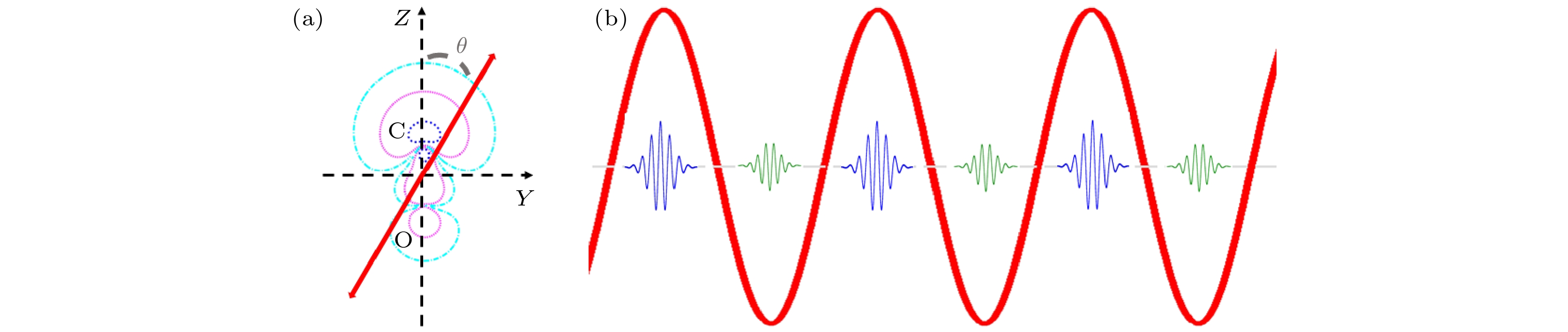
图 1 (a) 激光场与极性分子CO的几何关系示意图, 其中激光偏振(红色双箭头)与分子轴(沿Z轴)的夹角为
$ \theta $ ; (b) 当激光偏振沿分子轴方向(即$ \theta = {0^ \circ } $ )时, 在单色场(红色粗实线)的作用下, CO分子每半个激光周期产生的阿秒脉冲(蓝色和绿色细实线)Fig. 1. (a) The geometric relation of the laser field and polar molecule CO, where
$ \theta $ is the angle between the molecular (Z) axis and the driving laser polarization (red double arrow); (b) attosecond bursts (blue and green thin solid lines) generated every half cycle of a monochromatic field (red thick line) from polar molecule CO when$ \theta = {0^ \circ } $ .
图 2 当激光偏振沿分子轴方向时, CO分子产生的高次谐波谱(a)及其对应的时频分析(b)
Fig. 2. High harmonic spectrum (a) and the corresponding time-frequency analysis (b) of CO molecules, when the laser polarization is along the molecular axis.
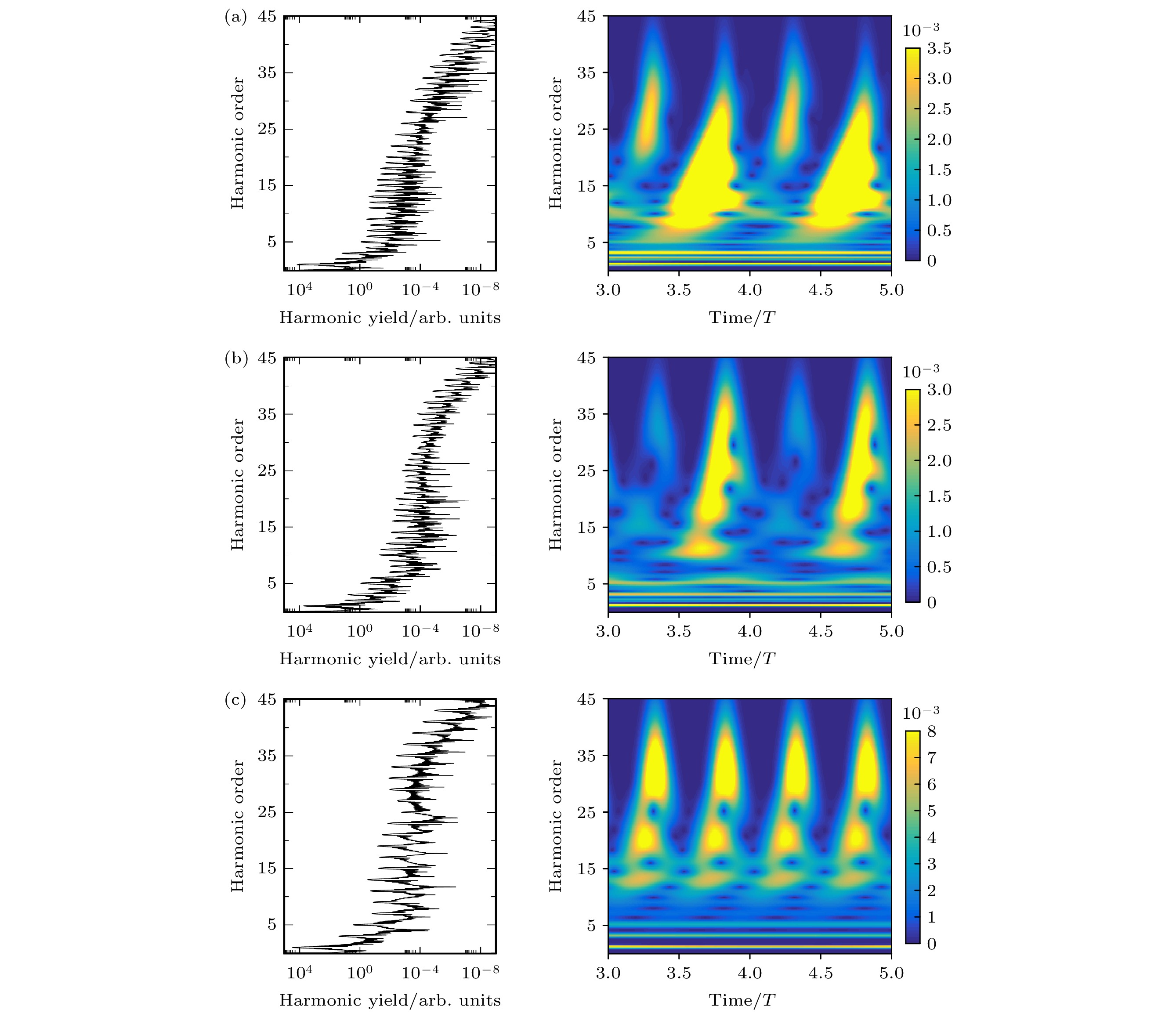
图 3 不同取向角
$ \theta $ 下, CO分子产生的高次谐波谱及其对应的时频分析 (a)$ \theta = {30^ \circ } $ ; (b)$ \theta = {60^ \circ } $ ; (c)$ \theta = {90^ \circ } $ . 除$ \theta $ 外, 其他计算参数同图2保持一致, 其中$ \theta $ 为分子轴与激光偏振的夹角, 如图1(a)所示Fig. 3. High harmonic spectra and corresponding time-frequency analyses at (a)
$ \theta = {30^ \circ } $ $ \theta $ , (b)$ \theta = {60^ \circ } $ and (c)$ \theta = {90^ \circ } $ . Note all parameters remain the same with Fig. 2; except for$ \theta $ , where$ \theta $ is the angle between the molecular axis and the driving laser polarization as shown in Fig.1 (a).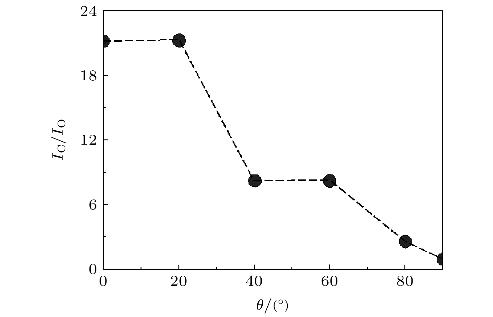
图 4 IC/IO随着取向角θ的变化关系, 其中IC(或IO)代表从C侧(或O侧)电离电子所辐射的谐波强度. 谐波强度的积分范围为H7阶到H50阶
Fig. 4. IC/IO as a function of the
$ \theta $ . IC (or IO) denotes the harmonic intensity emitted by the electrons ionized from C (or O) side with an integration range from H7th to H50th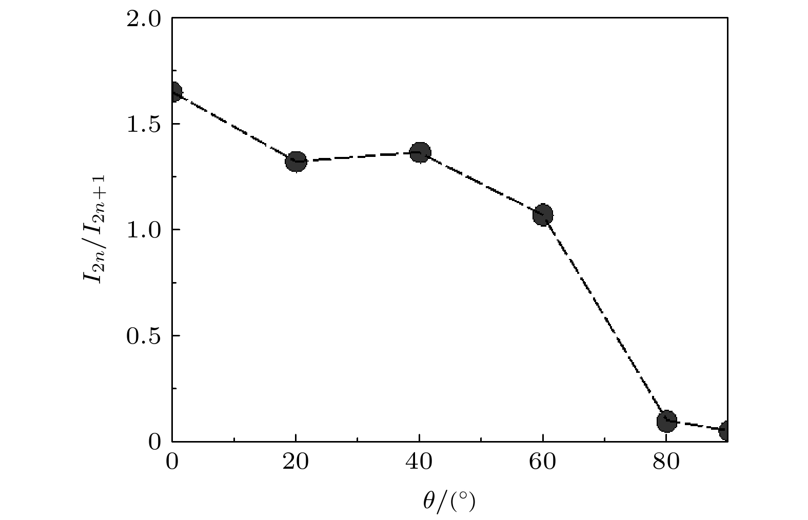
图 5 平台区的偶次和奇次谐波的强度比I2n/I2n+1随着取向角θ的变化关系, 其中I2n(或I2n+1)表示对H7到H50阶谐波中偶(或奇)次谐波的强度积分结果
Fig. 5. The intensity ratio of even and odd order harmonics I2n/I2n+1 versus the alignment angle θ, where I2n (or I2n+1) represents the integrated intensity of even (or odd) order harmonics with a frequency range from H7th to H50th.

图 6 沿O(黑色实线)和C(红色虚线)两侧的最外层轨道的光电离截面, 该结果由ePloyScat程序计算所得
Fig. 6. Photoionization cross sections of the HOMO from O side (black solid line) and C side (red dotted line), which are simulated by ePloyScat.
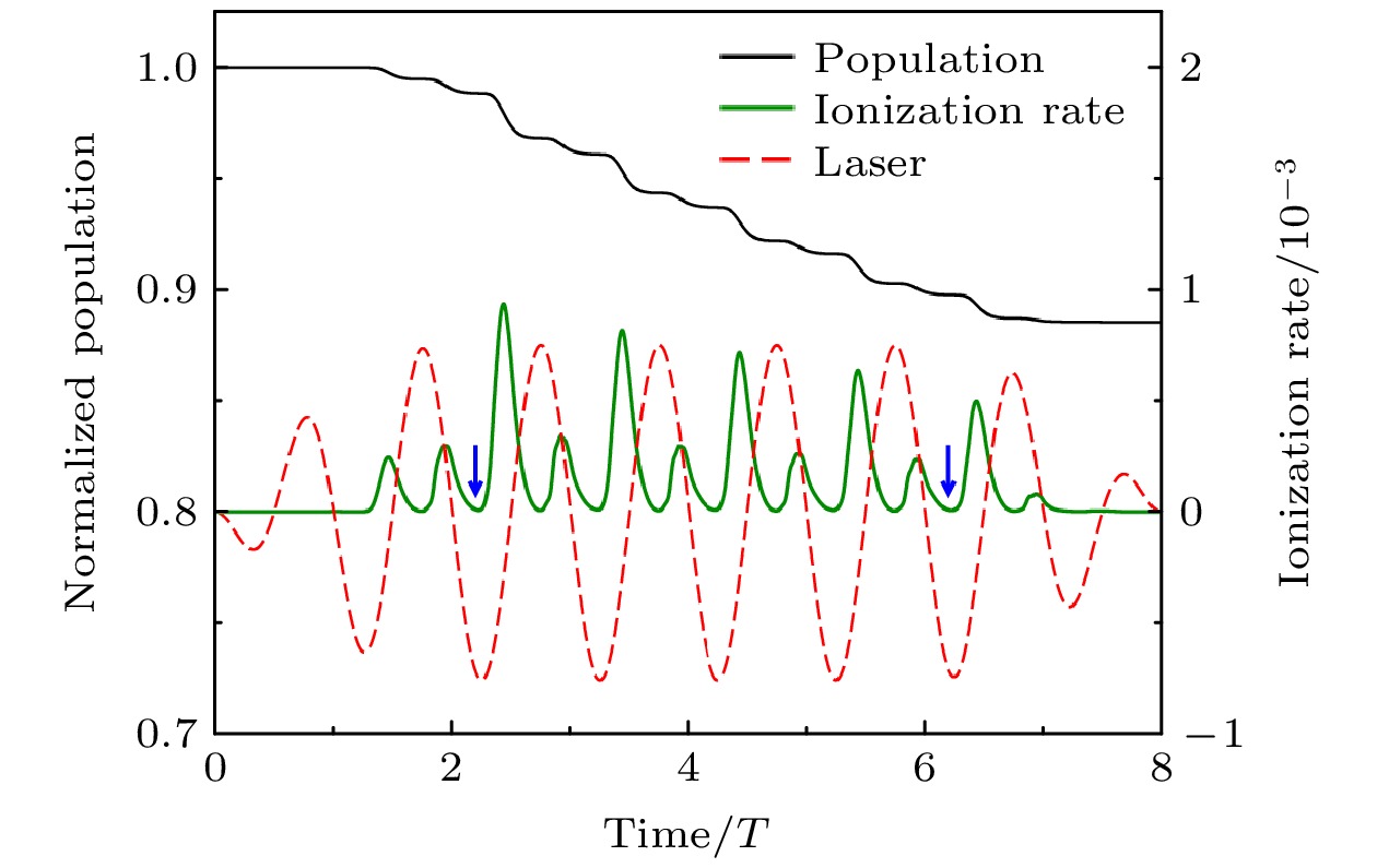
图 7 归一化的电子占据数(黑色实线)和电离速率(绿色实线)随着时间的变化关系. 红色虚线为激光场, 蓝色箭头所示的区域为激光脉冲的平台区
Fig. 7. Time profile of normalized population (black solid line) and ionization rates (green solid line) of electrons. The red dotted line denotes the used laser field. The time range marked by blue arrows is the plateau region of the used laser field.
-
[1] McPherson A, Gibson G, Jara H, Johann U, Luk T S, McIntyre I A, Boyer K, Rhodes C K 1987 J. Opt. Soc. Am. B: Opt. Phys. 4 595
Google Scholar
[2] Ferray M, L'Huillier A, Li X F, Lompre L A, Mainfray G, Manus C 1988 J. Phys. B: At. Mol. Opt. Phys. 21 L31
Google Scholar
[3] Brabec T, Krausz F 2000 Rev. Mod. Phys. 72 545
Google Scholar
[4] Krausz F, Ivanov M 2009 Rev. Mod. Phys. 81 163
Google Scholar
[5] Pazourek R, Nagele S, Burgdörfer J 2015 Rev. Mod. Phys. 87 765
Google Scholar
[6] Mourou G 2019 Rev. Mod. Phys. 91 030501
Google Scholar
[7] Krause J L, Schafer K J, Kulander K C 1992 Phys. Rev. Lett. 68 3535
Google Scholar
[8] Corkum P B 1993 Phys. Rev. Lett. 71 1994
Google Scholar
[9] Lewenstein M, Balcou P, Ivanov M Y, L’Huillier A, Corkum P B 1994 Phys. Lett. A 49 2117
Google Scholar
[10] Yang Y, Liu L, Zhao J, Tu Y, Liu J, Zhao Z 2021 J. Phys. B:At. Mol. Opt. Phys. 54 144009
Google Scholar
[11] Huang Y, Zhao J, Shu Z, Zhu Y, Liu J, Dong W, Wang X, Lü Z, Zhang D, Yuan J, Chen J, Zhao Z 2021 Ultrafast Science 2021 9837107
Google Scholar
[12] Li L, Zhang Y, Lan P, Huang T, Zhu X, Zhai C, Yang K, He L, Zhang Q, Cao W, Lu P 2021 Phys. Rev. Lett. 126 187401
Google Scholar
[13] Ghimire S, Reis D A 2019 Nat. Phys. 15 10
Google Scholar
[14] Liu L, Zhao J, Dong W, Liu J, Huang Y, Zhao Z 2017 Phys. Lett. A 96 053403
Google Scholar
[15] Liu L, Zhao J, Yuan J M, Zhao Z X 2019 Chin. Phys. B 28 114205
Google Scholar
[16] Luu T T, Yin Z, Jain A, Gaumnitz T, Pertot Y, Ma J, Wörner H J 2018 Nat. Commun. 9 3723
Google Scholar
[17] Zeng A W, Bian X B 2020 Phys. Rev. Lett. 124 203901
Google Scholar
[18] Hu H, Li N, Liu P, Li R, Xu Z 2017 Phys. Rev. Lett. 119 173201
Google Scholar
[19] Ren Z, Yang Y, Zhu Y, Zan X, Zhao J, Zhao Z 2021 J. Phys. B: At. Mol. Opt. Phys. 54 185601
Google Scholar
[20] Vos J, Cattaneo L, Patchkovskii S, Zimmermann T, Cirelli C, Lucchini M, Kheifets A, Landsman A S, Keller U 2018 Science 360 1326
Google Scholar
[21] Zhang B, Yuan J, Zhao Z 2015 Comput. Phys. Commun. 194 84
Google Scholar
[22] Zhang B, Yuan J, Zhao Z 2013 Phys. Rev. Lett. 111 163001
Google Scholar
[23] Zhang B, Yuan J, Zhao Z 2014 Phys. Rev. A 90 035402
Google Scholar
[24] Zhang B, Zhao J, Zhao Z 2018 Chin. Phys. Lett. 35 043201
Google Scholar
[25] Kobus J 1993 Chem. Phys. Lett. 202 7
Google Scholar
[26] Dong W, Hu H, Zhao Z 2020 Opt. Express 28 22490
Google Scholar
[27] Zhang B, Lein M 2019 Phys. Rev. A 100 043401
Google Scholar
[28] Le C T, Vu D D, Ngo C, Le V H 2019 Phys. Rev. A 100 053418
Google Scholar
[29] Kraus P M, Baykusheva D, Wörner H J 2014 Phys. Rev. Lett. 113 023001
Google Scholar
[30] Frumker E, Kajumba N, Bertrand J B, Wörner H J, Hebeisen C T, Hockett P, Spanner M, Patchkovskii S, Paulus G G, Villeneuve D M, Naumov A, Corkum P B 2012 Phys. Rev. Lett. 109 233904
Google Scholar
[31] 徐克尊 2012 高等原子分子物理学 第3版 (合肥: 中国科学技术大学出版社) 第51—52页
Xu K Z 2012 Advanced Atomic and Molecular Physics (3rd Ed.) (Hefei: University of Science and Technology of China Press) pp51—52 (in Chinese)
[32] Antoine P, Piraux B, Maquet A 1995 Phys. Lett. A 51 R1750
[33] Shu Z, Liang H, Wang Y, Hu S, Chen S, Xu H, Ma R, Ding D, Chen J 2022 Phys. Rev. Lett. 128 183202
Google Scholar
[34] 刘璐, 赵晶, 袁建民, 赵增秀 2017 中国科学: 物理学 力学 天文学 047 033006
Google Scholar
Liu L, Zhao J, Yuan J M, Zhao Z X 2017 Sci Sin-Phys. Mech. Astron. 047 033006
Google Scholar
[35] Chen Y J, Fu L B, Liu J 2013 Phys. Rev. Lett. 111 073902
Google Scholar
[36] Huang Y, Meng C, Wang X, Lü Z, Zhang D, Chen W, Zhao J, Yuan J, Zhao Z 2015 Phys. Rev. Lett. 115 123002
Google Scholar
[37] Gianturco F A, Lucchese R R, Sanna N 1994 J. Chem. Phys. 100 6464
Google Scholar
[38] Natalense A P P, Lucchese R R 1999 J. Chem. Phys. 111 5344
Google Scholar
-
[1] 张春艳. H离子团簇高次谐波平台展宽与团簇膨胀. 物理学报, 2023, 72(21): 214203. doi: 10.7498/aps.72.20230534 [2] 于术娟, 刘竹琴, 李雁鹏. 对称分子 ${\text{H}}_{\text{2}}^{\text{ + }}$ 在强短波激光场中高次谐波椭偏率性质的研究. 物理学报, 2023, 72(4): 043101. doi: 10.7498/aps.72.20221946[3] 姚惠东, 崔波, 马思琦, 余超, 陆瑞锋. 原子错位堆栈增强双层MoS2高次谐波产率. 物理学报, 2021, 70(13): 134207. doi: 10.7498/aps.70.20210731 [4] 袁长全, 郭迎春, 王兵兵. 准直的O2分子高次谐波谱中的干涉效应. 物理学报, 2021, 70(20): 204206. doi: 10.7498/aps.70.20210433 [5] 范鑫, 梁红静, 单立宇, 闫博, 高庆华, 马日, 丁大军. 基于高次谐波产生的极紫外偏振涡旋光. 物理学报, 2020, 69(4): 044203. doi: 10.7498/aps.69.20190834 [6] 李夏至, 邹德滨, 周泓宇, 张世杰, 赵娜, 余德尧, 卓红斌. 等离子体光栅靶的表面粗糙度对高次谐波产生的影响. 物理学报, 2017, 66(24): 244209. doi: 10.7498/aps.66.244209 [7] 管仲, 李伟, 王国利, 周效信. 激光驱动晶体发射高次谐波的特性研究. 物理学报, 2016, 65(6): 063201. doi: 10.7498/aps.65.063201 [8] 李贵花, 谢红强, 姚金平, 储蔚, 程亚, 柳晓军, 陈京, 谢新华. 中红外飞秒激光场中氮分子高次谐波的多轨道干涉特性研究. 物理学报, 2016, 65(22): 224208. doi: 10.7498/aps.65.224208 [9] 罗香怡, 刘海凤, 贲帅, 刘学深. 非均匀激光场中氢分子离子高次谐波的增强. 物理学报, 2016, 65(12): 123201. doi: 10.7498/aps.65.123201 [10] 余朝, 孙真荣, 郭东升. 高次谐波的Guo-Åberg-Crasemann理论及其截断定律. 物理学报, 2015, 64(12): 124207. doi: 10.7498/aps.64.124207 [11] 李雁鹏, 于术娟, 陈彦军. 不同取向角下CO2分子波长依赖的垂直谐波效率. 物理学报, 2015, 64(18): 183102. doi: 10.7498/aps.64.183102 [12] 陈高, 杨玉军, 郭福明. 晶体环境下高次谐波谱的截止频率分析. 物理学报, 2013, 62(8): 083202. doi: 10.7498/aps.62.083202 [13] 王学昭, 沈容, 路阳, 纪爱玲, 孙刚, 陆坤权, 崔平. 极性分子型电流变液导电机理研究. 物理学报, 2010, 59(10): 7144-7148. doi: 10.7498/aps.59.7144 [14] 崔磊, 王小娟, 王帆, 曾祥华. 脉冲激光偏振方向对氧分子高次谐波的影响——基于含时密度泛函理论的模拟. 物理学报, 2010, 59(1): 317-321. doi: 10.7498/aps.59.317 [15] 李会山, 李鹏程, 周效信. 强激光场中模型氢原子的势函数对产生高次谐波强度的影响. 物理学报, 2009, 58(11): 7633-7639. doi: 10.7498/aps.58.7633 [16] 施德恒, 刘玉芳, 孙金锋, 张金平, 朱遵略. 基态O和D原子的低能弹性碰撞及OD(X2Π)自由基的准确解析势与分子常数. 物理学报, 2009, 58(4): 2369-2375. doi: 10.7498/aps.58.2369 [17] 洪伟毅, 曹 伟, 兰鹏飞, 陆培祥. 静电场对高次谐波时频特性的影响. 物理学报, 2007, 56(11): 6623-6628. doi: 10.7498/aps.56.6623 [18] 顾 斌, 崔 磊, 曾祥华, 张丰收. 超强飞秒激光脉冲作用下氢分子的高次谐波行为——基于含时密度泛函理论的模拟. 物理学报, 2006, 55(6): 2972-2976. doi: 10.7498/aps.55.2972 [19] 崔 磊, 顾 斌, 滕玉永, 胡永金, 赵 江, 曾祥华. 脉冲激光偏振方向对氮分子高次谐波的影响--基于含时密度泛函理论的模拟. 物理学报, 2006, 55(9): 4691-4694. doi: 10.7498/aps.55.4691 [20] 王大威, 刘婷婷, 杨宏, 蒋红兵, 龚旗煌. 介质的非均匀性对高次谐波影响的研究. 物理学报, 2002, 51(9): 2034-2037. doi: 10.7498/aps.51.2034


 下载:
下载:


计量
- 文章访问数: 8512
- PDF下载量: 168
- 被引次数: 0
