1.   引　言

非视域(non-line-of-sight, NLOS)成像是对视线外的隐藏物体进行光学探测和可视化的新兴技术, 类似于“视线拐弯”或“隔墙观物”^[1-7]. 在机器视觉、制造业、医学成像、自动驾驶、军事反恐等领域具有广阔的应用前景. NLOS基于飞行时间探测技术, 主动向一个中介反射面发射激光, 利用探测器捕获从隐藏物体上发生散射返回的光子的空间时间信息来重建隐藏物体的形状^[8].

近年来, 非视域成像技术成为研究热点之一. 2012年, Velten等^[9]使用条纹相机和超快激光器搭建非视域成像系统, 并提出了一种椭圆反投影算法对隐藏物体进行三维重建. 2016年, Klein等^[10]提出了基于合成瞬态渲染的NLOS, 该研究将NLOS转化为了凸优化问题. 2018年, O’Toole等^[11]探索了一种适用于共焦NLOS系统的光锥变换反演法(the light-cone transform, LCT), LCT降低了重建复杂度. 2019年, Liu等^[5]提出了基于相量场虚拟波的NLOS, 将NLOS过程公式化为波成像问题, 可以将经典光学中成熟的见解和技术应用在NLOS领域, 即将NLOS成像系统模拟为一个虚拟的视线成像系统. 在NLOS定位和成像的研究中, 为了提高重建质量和效率, 除了对捕获的飞行时间信息进行滤波处理外^[12], 主要从三维重建算法、成像装置和中介反射面的选择等方面进一步改进, 如对反投影算法改进从而实现了多目标NLOS、远距离NLOS和快速反投影NLOS^[2,13-15]. 也有研究引入深度学习来解决NLOS问题^[16-19]. 在之前的研究中, 使用条纹相机、单光子雪崩二极管(single-photon avalanche diode , SPAD)、飞行时间(time of flight , TOF)相机等作为探测器做了大量研究^[9,20,21]. 2021年, 中国科学技术大学研究团队基于短激光脉冲泵浦技术构建了一个工作在近红外波段的上转换单光子探测器(up-conversion single-photon detector, UCSPD), 有效提高了探测器的时间分辨率^[7].

目前主流的NLOS是基于瞬态光传输进行研究的, 主要包括椭圆反投影方法、光锥变换反演法和凸优化法等. 椭圆反投影法对于存储和处理的要求较高, 并且接收到的回波信号弱^[9,13,14,20], 基于光锥变换的非视域成像通过使用共焦扫描系统解决了回波信号弱的问题. 光锥变换反演法将探测器捕获到的瞬态图像表示为一个三维卷积, 该卷积在变换域中模拟自由空间的光传输, 光锥变换提供了快速且高效的方式计算反向光传输. 可以将光锥变换反演法看作是反卷积的过程, 维纳滤波是经典的反卷积方法, 其中功率谱密度噪信比(power spectral density noise-to-signal ratio, PSDNSR)决定了重建成像的质量. 在非视域成像中每种隐藏场景的PSDNSR不同, 每次都需要调节, PSDNSR通常采用经验值或者反复尝试来获取. 该方法进行反卷积很难一步就找到最佳的PSDNSR, 需手动调节PSDNSR进行多次实验. 而快速地进行反卷积对非视域成像的实时应用至关重要, 因此本文重点研究改进的维纳滤波算法使光锥变换反演法更高效.

2.   基于光锥变换的非视域成像原理模型

本文同样使用光锥变换反演法进行非视域成像, 因此本文使用共焦光路, 实验设置如图1所示. 通过使用分束镜将激光发射光路与探测器接收光子的光路合成共焦非视域成像系统. 激光器向中介反射面发射脉冲激光, 经过三次散射后使用超导纳米线单光子探测系统(superconducting nanowire single-photon detector, SNSPD)作为探测器捕获返回的光子信息. 时间相关单光子计数 (time-correlated single-photon counting, TCSPC)模块对SNSPD捕获到的每个像素的光子数进行直方图统计, 得到瞬态图像.

图 1  实验场景示意图, 激光通过振镜对中介面扫描, 探测器接收来自中介面反射的直接光和来自隐藏物体的间接光

Fig. 1.  Experimental scene, the laser scans the intermediate surface through the galvanometer, and the detector receives direct light reflected from the intermediate surface and indirect light from a hidden object.

下载: 全尺寸图片 幻灯片

探测器捕获到的瞬态图像可以表示为^[11]

式中, $(x', y')$是激光照射在中介反射面上的点, $(x, y, z)$是隐藏物体表面上的点, $r$表示这两个点之间的距离. $\rho$是满足$z > 0$的三维半空间$\varOmega$中隐藏物体表面每个点的反照率, 函数$\delta$表示由${x^2} + {y^2} + {z^2} = {\left( { {{tc}}/{2}} \right)^2}$给出的时空四维超圆锥的表面.

对瞬态成像模型做变量代换后可以写成一个3D卷积: ${R_t}\{ g\} = h * {R_z}\{ \rho \}$. 其中, $h$表示移位不变的卷积核, 即$\delta \left( {2\sqrt {{{(x' - x)}^2} + {{(y' - y)}^2} + {z^2}} - tc} \right)$, ${R_t}$是对$g$沿$t$轴衰减及重采样, ${R_z}$是对$\rho$沿$z$轴衰减及重采样. 接下来, 对成像模型进行离散化, 在空间域中经变量代换和离散后的瞬态图像可以表示为

其中$\tilde g = {R_t}g$, $\tilde \rho = {R_z}\rho$, $\eta$是白噪声. $H$是卷积核$h$的离散化, 非视域成像的过程就是获取$\tilde \rho$的近似估计${\tilde \rho _ * }$.

维纳滤波是经典且有效的反卷积方法, 文献[11]正是使用维纳滤波反卷积, 最后得到隐藏物体的反照率为

其中, $\hat H(u, v, w)$为卷积核$H$的傅里叶变换, $G(u, v, w)$为瞬态图像$\tilde g$的傅里叶变换, $\varPi (u, v, w) = \dfrac{{{S_{\tilde \rho \tilde \rho }}(u, v, w)}}{{{S_{\eta \eta }}(u, v, w)}}$是瞬态图像的功率谱密度噪信比, 一般很难求出, 所以常用常数项$K$代替$\varPi (u, v, w)$, 得:

一般来说, $K$值的选取决定着非视域成像的质量, 通常采用经验值或反复尝试来手动调节, 但该方法成像效率不高. 并且常数项$K$值代替$\varPi (u, v, w)$进行维纳滤波时, 没有用到足够的先验知识, 导致难以快速找到最佳值. 因此本文引入瞬态图像中频域的方法实现对$K$的快速计算.

3.   基于中频域维纳滤波的非视域成像算法

瞬态图像的频谱$G(u, v, w)$是一个$M \times N \times P$的复数矩阵, 如图2所示为$w = 50$时瞬态图像的频谱图$\left| {G(u, v, w)} \right|$. 可见瞬态图像的大部分信息分布在频谱原点$G(u, v, w) = (0, 0, 50)$附近的“低频”区域, 卷积核的信息被完全淹没在瞬态图像的信息中, 而频谱的“高频”区域幅度小且易被噪声污染. 由于“低频”和“高频”区域的频谱幅度相差大, 不会出现交叠, 两者之间必然存在一个中间过渡区域, 即不含太多的瞬态图像能量又没有被噪声淹没, 将之称为“中频域”, 可以用于估计$K$值从而进行维纳滤波反卷积^[22]. 非视域成像系统中捕获的瞬态图像中大多数信号变化缓慢, 只有少数信号变化大, 频谱往往为全局单减, 因此瞬态图像存在中频域并且数值特征大都相似.

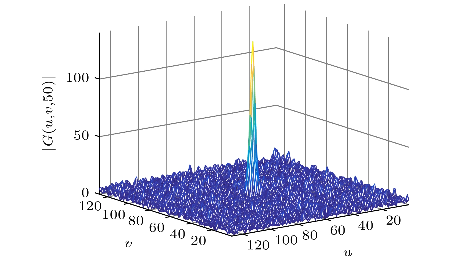
图 2  $w = 50$时瞬态图像的频谱图$\left| {G(u, v, w)} \right|$

Fig. 2.  Spectrum $\left| {G(u, v, w)} \right|$ of the transient image at$w = 50$.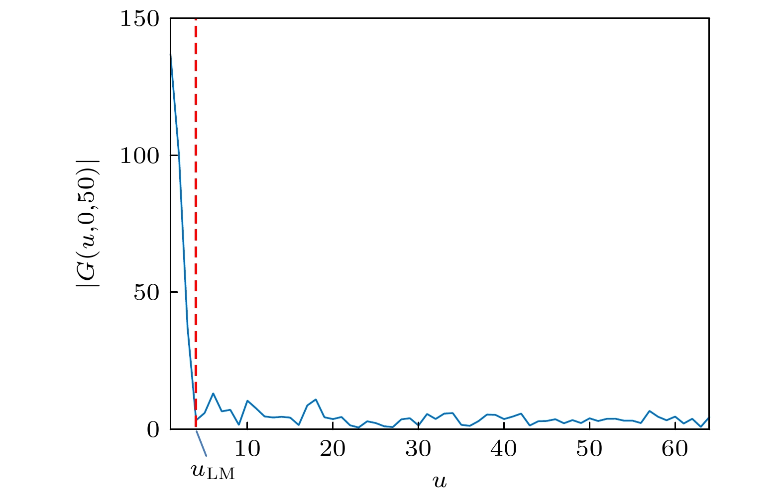

下载: 全尺寸图片 幻灯片

如图3所示, 取$w = 50$时瞬态图像的幅度$\left| {G(u, v, w)} \right|$中过原点的一条线$\left| {G(u, 0, 50)} \right|$, $G(u, 0, 50)$是共轭对称的, 所以只考虑前半个周期$u \in {U_{\text{T}}} = [0, {u_{\text{T}}}]$上的值, 其中${u_{\text{T}}}{\text{ = }}\left\lfloor {(P - 1)/2} \right\rfloor$, $\lfloor ·\rfloor$表示向零取整. 那么低频域位于$u = 0$附近, 高频域位于$u = {u_{\text{T}}}$附近. 通常该曲线中有两个明显的全局转折点, 即中频域的边界点. 因为低频域聚集了瞬态图像的大部分信息, 所以在曲线$\left| {G(u, 0, 50)} \right|$中可以看到一个清晰的转折点${u_{{\text{LM}}}}$, 即低频域和中频域的分界点. 而高频域的值很小且被近似均匀分布的噪声所污染, 所以可以在曲线$\ln \left| {G(u, 0, 50)} \right|$中看到另一个清晰的转折点${u_{{\text{MH}}}}$, 即中频域和高频域的转折点. 但是, 由于$\ln \left| {G(u, 0, 50)} \right|$通常是剧烈振荡的, 有很多局部转折点, 很难正确找到${u_{{\text{MH}}}}$, 因此将曲线$\ln \left| {G(u, 0, 50)} \right|$平滑之后得到${G_r}(u)$来计算转折点${u_{{\text{MH}}}}$. 如图4所示, 根据曲线${G_r}(u)$的几何特性, 过$(0, {G_r}(0))$和$({u_{\text{T}}}, {G_r}({u_{\text{T}}}))$两点作直线, 那么${G_r}(u)$上距离该直线最远的距离就是${u_{{\text{MH}}}}$, 因此可以计算出${u_{{\text{MH}}}}$为

图 3  幅度$\left| {G(u, v, w)} \right|$中过原点的一条线$\left| {G(u, 0, 50)} \right|$

Fig. 3.  A line $\left| {G(u, 0, 50)} \right|$ through the origin in the spectral magnitude $\left| {G(u, v, w)} \right|$.

下载: 全尺寸图片 幻灯片

图 4  幅度$\ln \left| {G(u, 0, 50)} \right|$平滑之后的曲线${G_r}(u)$

Fig. 4.  Curve ${G_r}(u)$ after amplitude $\ln \left| {G(u, 0, 50)} \right|$ smoothing.

下载: 全尺寸图片 幻灯片

利用中频域对维纳滤波反卷积公式中的$K$值进行估计如下. 首先选取一条过原点线$\big| {\hat H(u, 0, 0)} \big|$, 令:

这时, 对$K$值的估计问题就转换为了获取$K$值使得${T_1}(u)$在抑制噪声的基础上最接近${T_0}(u)$. 因为低频域和中频域中的噪声很小可以忽略, 有${T_0}(u) \approx {T_{\text{1}}}(u) \approx {T_2}(u), u \in {U_{{\text{LM}}}}$, 其中${U_{{\text{LM}}}}$为低频域和中频域. 在高频域中, 噪声近似为均匀分布, 有${T_0}(u) \approx {T_{\text{0}}}({u_{{\text{MH}}}}), u \in {U_{\text{H}}}$. 为了抑制噪声的影响, 使${T_1}(u) \geqq {T_0}(u)$在高频区域成立, 即:

其中, ${U_{\text{H}}}$为高频域. 因此, 引入调节参数$\eta$, 利用${T_0}(u)$和${T_1}(u)$的表达式即可解得$K$值^[22]:

其中$u \in {U_{\text{T}}} = [0, {u_{\text{T}}}]$, 上述引入的参数$\eta$称为“噪声抑制参数”, 用来调节噪声和图像细节的平衡.

上文利用空间维度上瞬态图像的频谱图$\left| {G(u, v, w)} \right|$的中频域来估计$K$值. 分析时间维度上瞬态图像的频谱图, 如图5所示为$u = 0$时瞬态图像的频谱图$\left| {G(u, v, w)} \right|$. 取幅度$\left| {G(u, v, w)} \right|$过原点的一条线$\left| {G(0, 0, w)} \right|$, 如图6所示, 也可计算出该曲线的中高频转折点${w_{{\text{MH}}}}$:

图 5  $u = 0$时瞬态图像的频谱图$\left| {G(u, v, w)} \right|$

Fig. 5.  Spectrum $\left| {G(u, v, w)} \right|$ of the transient image at$u = 0$.

下载: 全尺寸图片 幻灯片

图 6  幅度$\left| {G(u, v, w)} \right|$中过原点的一条线$\left| {G(0, 0, w)} \right|$

Fig. 6.  A line $\left| {G(0, 0, w)} \right|$ through the origin in the spectral magnitude $\left| {G(u, v, w)} \right|$.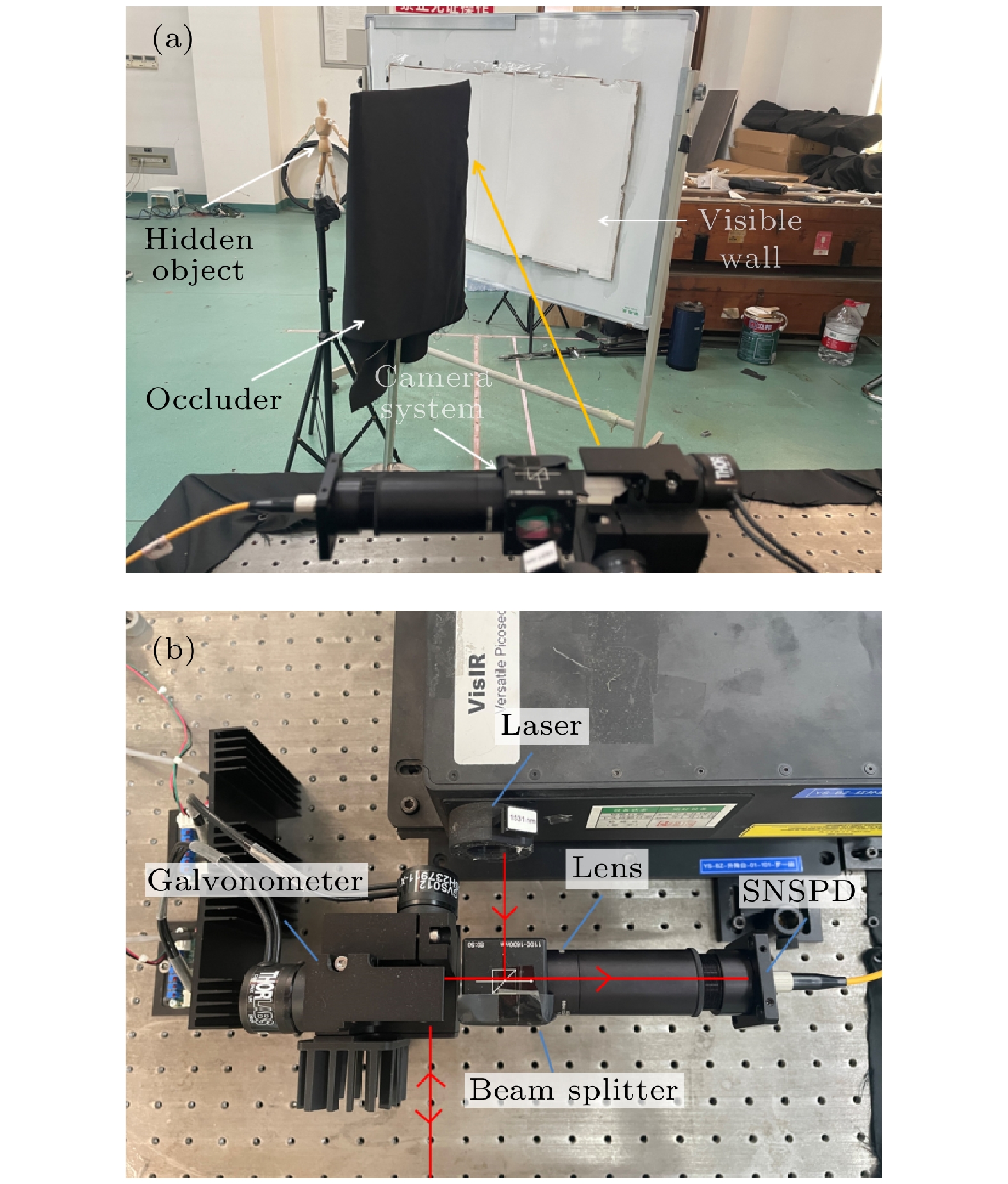

下载: 全尺寸图片 幻灯片

其中$w \in {W_{\text{T}}} = [0, {w_{\text{T}}}]$是曲线$\left| {G(0, 0, w)} \right|$的前半周期, ${G_r}(w)$是曲线$\ln \left| {G(0, 0, w)} \right|$平滑之后的曲线.

同理对$K$值进行估计:

其中$w \in {W_{\text{T}}} = [0, {w_{\text{T}}}]$.

分别使用空间维度上的频谱图和时间维度上的频谱图估计的$K$值没有很大的差异, 本文选择使用时间维度上的频谱图$\left| {G(0, 0, w)} \right|$对$K$值进行估计.

针对基于光锥变换的非视域成像问题, 使用基于中频域的维纳滤波算法对$K$值进行估计并完成重建的步骤如下:

1)在共焦非视域成像系统中, 使用探测器捕获瞬态图像$g(x', y', t)$;

2)对经过变量代换的瞬态图像$\tilde g$进行傅里叶变换得到频谱$G(u, v, w)$;

3)计算出曲线$\ln \left| {G(0, 0, w)} \right|$, 再对该曲线平滑得到${G_r}(w)$;

4)根据(11)式计算出${w_{{\text{MH}}}}$;

5)根据(12)式计算出$K$值;

6)使用维纳滤波算法对瞬态图像反卷积并进行傅里叶反变换得到${\tilde \rho _{\text{*}}}$;

7)最终使用(4)式得到隐藏物体表面的反照率${\rho _*}$.

4.   实验及结果分析

搭建的实验场景如图7所示, 该共焦非视域成像系统包含的光源为波长1530 nm的激光脉冲, 脉冲宽度为70 ps, 重复频率为40 MHz, 平均功率为750 mW. 采用的探测器为超导纳米线单光子探测系统(SNSPD), 其探测效率约为70%. 使用分束器(Thorlabs CCM1-BS015/M)将探测光路和激光发射光路共轴. 使用振镜(Thorlabs GVS012)来实现对中介面的扫描. 时间相关单光子计数模块以1 ps的时间分辨率对探测事件进行时间标记.

图 7  实验场景　(a)为在实验室搭建的共焦非视域成像场景; (b)为共焦非视域成像系统

Fig. 7.  Experimental scene: (a) The confocal non-horizontal imaging scene built in the laboratory; (b) demonstrates the confocal non-horizontal imaging system.

下载: 全尺寸图片 幻灯片

本文通过上述实验装置对如图8所示的5个隐藏场景捕获光子飞行时间信息, 5个隐藏场景分别为T形纸板、人偶模型手臂向下、房屋形纸板、C形纸板和人偶模型手臂向上.

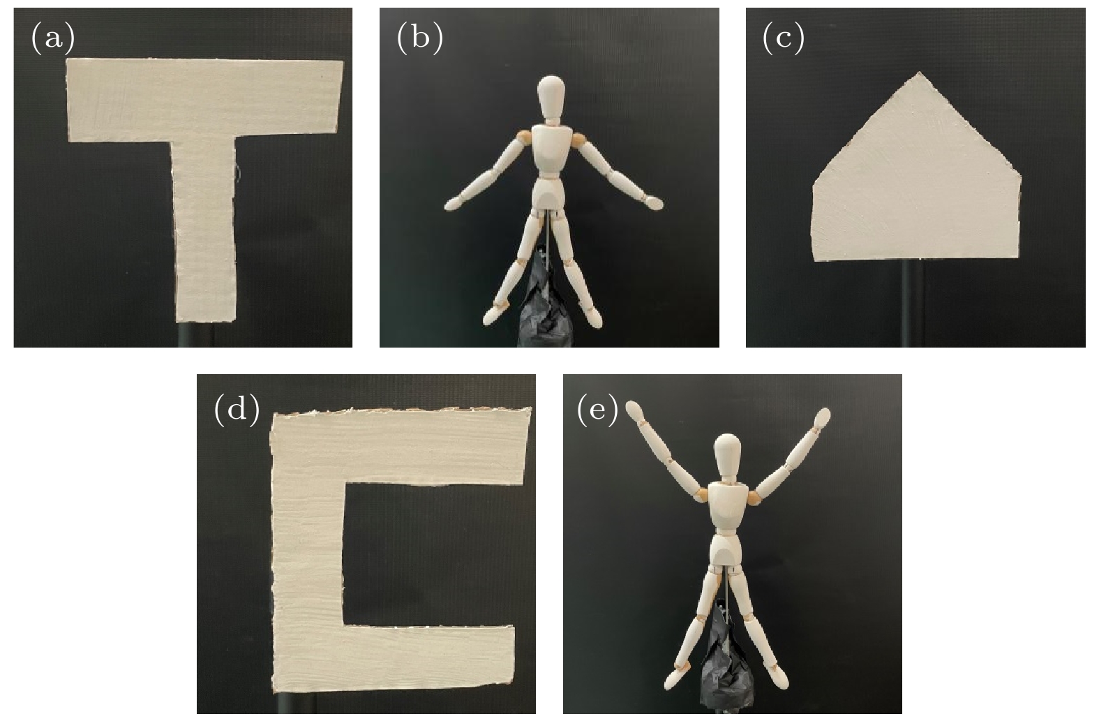
图 8  隐藏场景　(a) T形纸板; (b)人偶模型手臂向下; (c)房屋形纸板; (d)C形纸板; (e)人偶模型手臂向上

Fig. 8.  Hidden scene: (a) T-shaped cardboard; (b) puppet model with arms down; (c) house-shaped cardboard; (d) C- shaped cardboard; (e) puppet model with arms up.

下载: 全尺寸图片 幻灯片

(12)式中的参数$\eta$用来调节噪声和图像的细节, 噪声和图像的清晰度会随$\eta$减小而变弱. 在评估了噪声大小的基础上, 本文选择$\eta = 1.1$来对K值进行估计, 此时噪声在可接受范围内且细节更加丰富. 基于中频域的维纳滤波算法对T形纸板、人偶模型手臂向下、房屋形纸板、C形纸板和人偶模型手臂向上5个隐藏场景K值的估计值分别为2.8678, 1.2353, 3.6711, 0.8096和1.5939.

为了说明本文算法对非视域成像的有效性, 分别取$K$为0.01, 0.1, 1, 10, 100, 1000对隐藏场景进行重建, 将传统维纳滤波的重建结果与基于中频域的维纳滤波得到的结果进行对比. 为方便起见, 只对比重建结果的正视图, 见图9—图18.

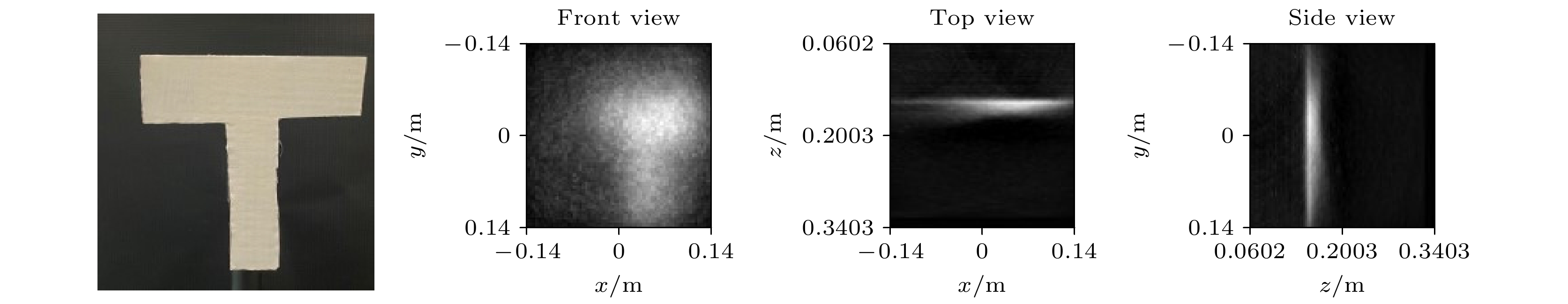
图 9  隐藏物体T形纸板和基于中频域的维纳滤波的重建结果

Fig. 9.  T-shaped cardboard and reconstruction results of NLOS imaging based on mid-frequency Wiener filtering.

下载: 全尺寸图片 幻灯片

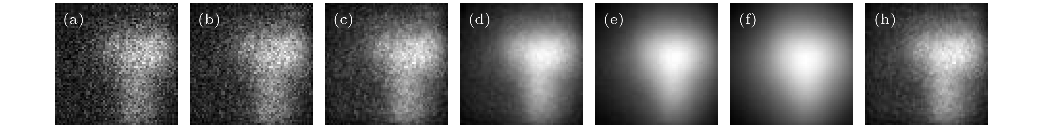
图 10  传统维纳滤波的重建结果与基于中频域的维纳滤波的重建结果对比　(a)−(f) T形纸板的隐藏场景分别取K为0.01, 0.1, 1, 10, 100, 1000进行维纳滤波复原的结果; (h) T形纸板基于中频域的维纳滤波重建的结果, 估出K为2.8678

Fig. 10.  Comparison between the reconstruction results of traditional Wiener filtering and the reconstruction results based on Wiener filtering in the mid-frequency domain: (a)−(f) The results of Wiener filtering reconstruction with K as 0.01, 0.1, 1, 10, 100, and 1000 for T-shaped cardboard respectively; (h) the reconstruction result of T-shaped cardboard using the NLOS imaging algorithm based on Wiener filtering of mid-frequency domain, and the estimated K is 2.8678.

下载: 全尺寸图片 幻灯片

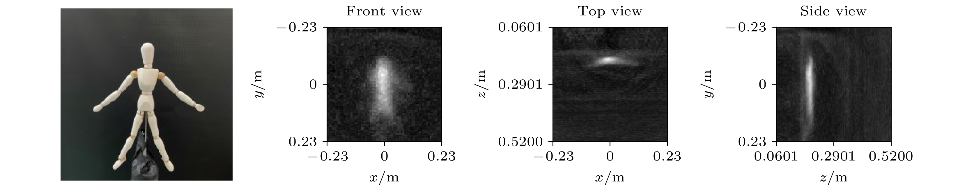
图 11  隐藏场景人偶模型手臂向下和基于中频域的维纳滤波的重建结果

Fig. 11.  Puppet model with arms down and reconstruction results of NLOS imaging based on mid-frequency Wiener filtering.

下载: 全尺寸图片 幻灯片

图 12  传统维纳滤波的重建结果与基于中频域的维纳滤波的重建结果对比　(a)−(f)人偶模型隐藏场景分别取K为0.01, 0.1, 1, 10, 100, 1000进行维纳滤波复原的结果; (h)人偶模型隐藏场景基于中频域的维纳滤波重建的结果, 估计出的K为1.2353

Fig. 12.  Comparison between the reconstruction results of traditional Wiener filtering and the reconstruction results based on Wiener filtering in the mid-frequency domain: (a)−(f) The results of Wiener filtering reconstruction with K as 0.01, 0.1, 1, 10, 100, and 1000 for puppet model with arms down respectively; (h) the reconstruction result of puppet model with arms down using the NLOS imaging algorithm based on Wiener filtering of mid-frequency domain, and the estimated K is 1.2353.

下载: 全尺寸图片 幻灯片

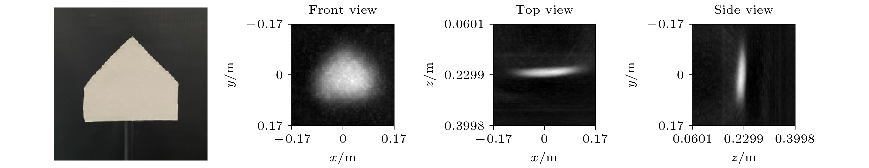
图 13  隐藏场景房屋形纸板和基于中频域的维纳滤波的重建结果

Fig. 13.  House-shaped cardboard and reconstruction results of NLOS imaging based on mid-frequency Wiener filtering.

下载: 全尺寸图片 幻灯片

图 14  传统维纳滤波的重建结果与基于中频域的维纳滤波的重建结果对比　(a)−(f)为房屋形纸板的隐藏场景分别取K为0.01, 0.1, 1, 10, 100, 1000进行维纳滤波复原的结果; (h)房屋形纸板隐藏场景基于中频域的维纳滤波重建的结果, 估计出的K为3.6711

Fig. 14.  Comparison between the reconstruction results of traditional Wiener filtering and the reconstruction results based on Wiener filtering in the mid-frequency domain: (a)−(f) The results of Wiener filtering reconstruction with K as 0.01, 0.1, 1, 10, 100, and 1000 for House-shaped cardboard respectively; (h) the reconstruction result of house-shaped cardboard using the NLOS imaging algorithm based on Wiener filtering of mid-frequency domain, and the estimated K is 3.6711.

下载: 全尺寸图片 幻灯片

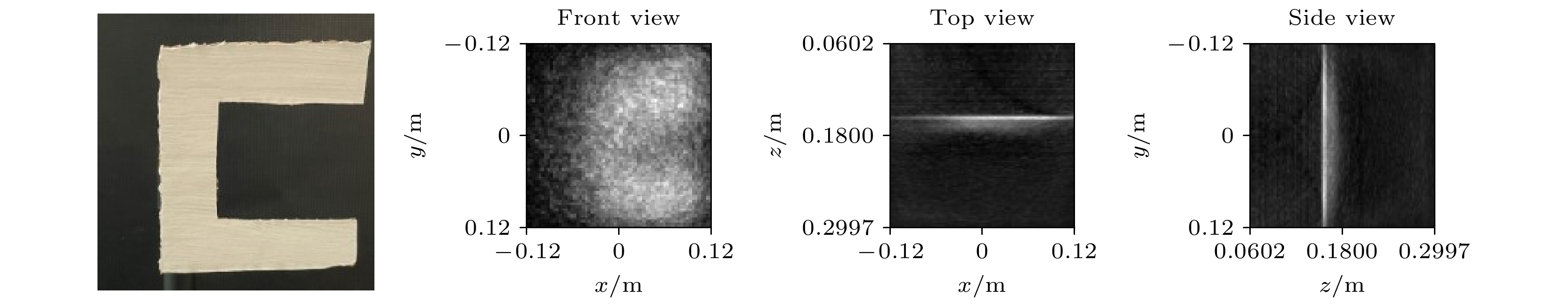
图 15  隐藏场景C形纸板和基于中频域的维纳滤波的重建结果

Fig. 15.  C- shaped cardboard and reconstruction results of NLOS imaging based on mid-frequency Wiener filtering.

下载: 全尺寸图片 幻灯片

图 17  隐藏场景人偶模型手臂向上和基于中频域的维纳滤波的重建结果

Fig. 17.  Puppet model with arms up and reconstruction results of NLOS imaging based on mid-frequency Wiener filtering.

下载: 全尺寸图片 幻灯片

图 18  传统维纳滤波的重建结果与基于中频域的维纳滤波的重建结果对比　(a)−(f)人偶模型手臂向上的隐藏场景分别取K为0.01, 0.1, 1, 10, 100, 1000进行维纳滤波复原的结果; (h)人偶模型手臂向上隐藏场景基于中频域的维纳滤波重建的结果, 估出的K为1.5939

Fig. 18.  Comparison between the reconstruction results of traditional Wiener filtering and the reconstruction results based on Wiener filtering in the mid-frequency domain: (a)−(f) The results of Wiener filtering reconstruction with K as 0.01, 0.1, 1, 10, 100, and 1000 for puppet model with arms up respectively; (h) the reconstruction result of puppet model with arms up using the NLOS imaging algorithm based on Wiener filtering of mid-frequency domain, and the estimated K is 1.5939.

下载: 全尺寸图片 幻灯片

考虑到人眼对于图像的主观评价不是从单一角度出发, 因此本文选择综合图像Tenengrad梯度和结构相似性(structural similarity, SSIM)两个指标来进行像质评价^[23], 从清晰度和空间结构性两方面来评价重建图像. 从图像像素的角度来看, 图像Tenengrad梯度GRAD越大, 图像内的边缘越清晰, 图像质量越好; 原始图像和重建图像的结构相似性越大, 重建效果越好, 图像质量越好. 考虑到图像Tenengrad梯度和SSIM两个指标的一致性和量级后, 通过线性加权, 得到最终图像评价指标为

式中, $\alpha$和$\beta$分别为图像Tenengrad梯度和SSIM的权值, $\alpha {\text{ + }}\beta {\text{ = 1}}$. 本文根据对重建图像的分析, 分别取$\alpha {\text{ = 0}}{\text{.1}}$, $\beta {\text{ = 0}}{\text{.9}}$. E_val越大, 图像质量越好, E_val越小, 图像质量越差. 图16所示为对不同$K$值维纳滤波的重建结果和基于中频域的维纳滤波重建结果的客观评价.

图 16  传统维纳滤波的重建结果与基于中频域的维纳滤波的重建结果对比　(a)−(f) C形纸板的隐藏场景分别取K为0.01, 0.1, 1, 10, 100, 1000进行维纳滤波复原的结果; (h) C形纸板隐藏场景基于中频域的维纳滤波重建的结果, 估出K值为0.8096

Fig. 16.  Comparison between the reconstruction results of traditional Wiener filtering and the reconstruction results based on Wiener filtering in the mid-frequency domain: (a)−(f) The results of Wiener filtering reconstruction with K as 0.01, 0.1, 1, 10, 100, and 1000 for C-shaped cardboard respectively; (h) the reconstruction result of C- shaped cardboard using the NLOS imaging algorithm based on Wiener filtering of mid-frequency domain, and the estimated K is 0.8096.

下载: 全尺寸图片 幻灯片

如图19所示, 本文方法计算出5个隐藏场景的$K$值分别在${\text{1}}{{\text{0}}^{\text{0}}}$, ${\text{1}}{{\text{0}}^{\text{0}}}$, ${\text{1}}{{\text{0}}^{\text{0}}}$, ${\text{1}}{{\text{0}}^{ - 1}}$, ${\text{1}}{{\text{0}}^{\text{0}}}$量级上. 基于中频域的维纳滤波算法取得的$K$值总能落在一个最佳的量级上, $K$值在该量级时, 图像综合质量评价值最高, 图像重建效果最好. 可以看出, 基于中频域维纳滤波的非视域成像算法重建图像的E_val值在一个较高的范围, 说明本文方法估计出的$K$值进行非视域成像得到的重建图像效果好, 并且速度更快. 实验结果表明, 使用本文方法能一步估出$K$值, 并且接近最佳值.

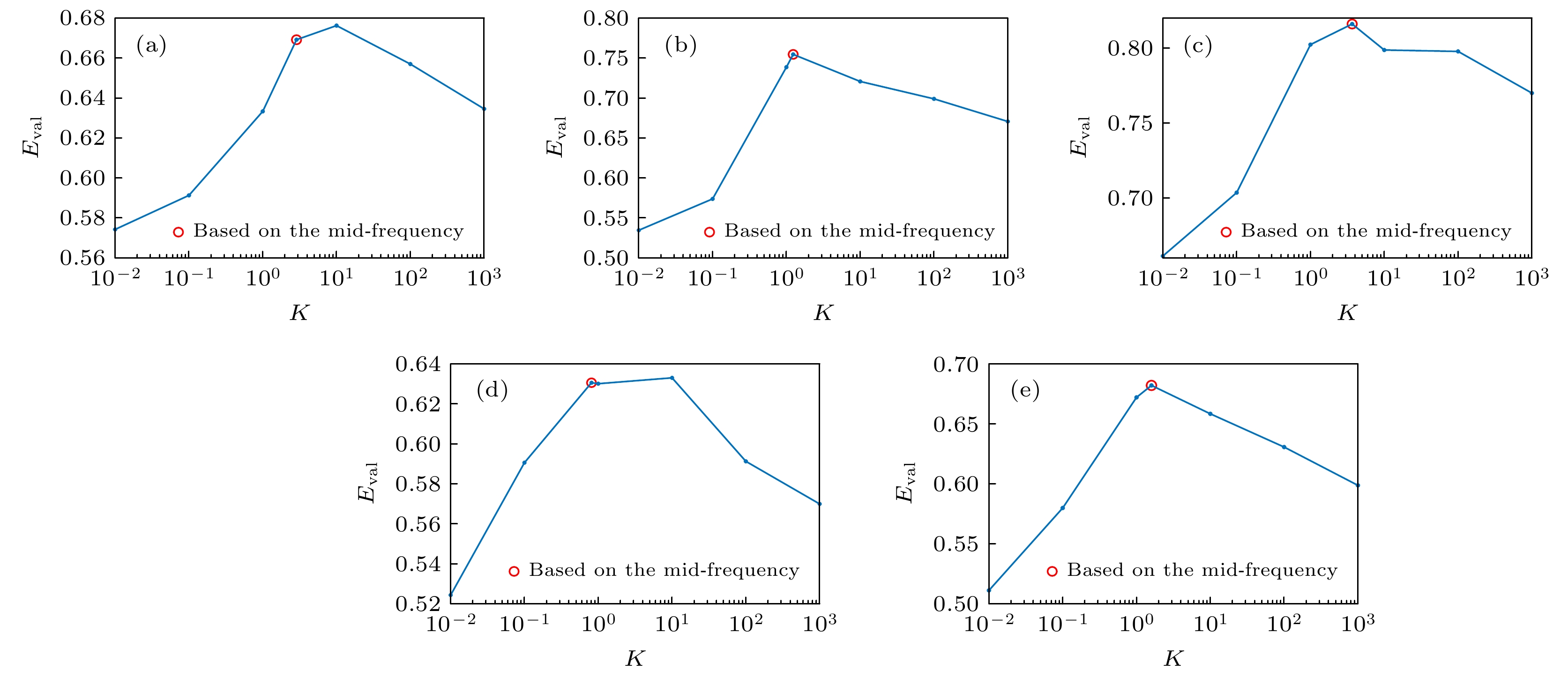
图 19  重建图像综合质量评价, 其中蓝色线为设置不同K得到的重建图像的综合质量评价值, 红色圆圈为基于中频域的维纳滤波重建图像的综合质量评价值　(a) T形纸板; (b)人偶模型手臂向下; (c)房屋形纸板; (d) C形纸板; (e)人偶模型手臂向上

Fig. 19.  Comprehensive quality evaluation of reconstructed images, the blue line is the comprehensive quality evaluation value of the reconstructed image obtained by setting different K, and the red circle is the comprehensive quality evaluation value of the reconstructed image based on the Wiener filter in the intermediate frequency domain: (a) The E_val of T-shaped cardboard, (b) the E_val of puppet model with arms down, (c) the E_val of house-shaped cardboard, (d) the E_val of C-shaped cardboard, (e) the E_val of puppet model with arms up.

下载: 全尺寸图片 幻灯片

5.   结　论

共焦光路中的非视域成像可以看作是一个反卷积问题, 在维纳滤波反卷积的过程中参数$K$值的选取对成像的速度以及重建的质量有很大的影响, 非视域成像中每种隐藏场景的最优$K$值都不一样, 每次实验都需人为调节. 针对该问题本文引入了基于中频域的非视域成像算法, 可以使用瞬态图像的中频域信息来估计$K$值. 相比其他取$K$值的算法, 该算法没有迭代和矩阵运算, 计算复杂度低, 能够快速的确定$K$值. 为了验证本文算法的有效性, 本文进行共焦非视域成像实验, 将一系列手动设置的$K$值的重建结果与基于中频域的非视域成像算法得到的重建结果进行了对比. 实验结果表明, 基于中频域的维纳滤波算法取得的$K$值能落在成像效果接近最佳的量级上. 综上, 该算法具有快速、准确和参数少的特点, 有效提升了共焦非视域成像的重建质量和实时性.