


-
自动微分是利用计算机自动化求导的技术, 最近几十年因为它在机器学习研究中的应用而被很多人了解. 如今越来越多的科学工作者意识到, 高效、自动化的求导可以为很多科学问题的求解提供新的思路, 其中自动微分在物理模拟中的应用尤为重要, 而且具有挑战性. 物理系统的可微分模拟可以帮助解决混沌理论、电磁学、地震学、海洋学等领域中的很多重要问题, 但又因为其对计算时间和空间的苛刻要求而对自动微分技术本身提出了挑战. 本文回顾了将自动微分技术运用到物理模拟中的几种方法, 并横向对比它们在计算时间、空间和精度方面的优势和劣势. 这些自动微分技术包括伴随状态法, 前向自动微分, 后向自动微分, 以及可逆计算自动微分.Automatic differentiation is a technology to differentiate a computer program automatically. It is known to many people for its use in machine learning in recent decades. Nowadays, researchers are becoming increasingly aware of its importance in scientific computing, especially in the physics simulation. Differentiating physics simulation can help us solve many important issues in chaos theory, electromagnetism, seismic and oceanographic. Meanwhile, it is also challenging because these applications often require a lot of computing time and space. This paper will review several automatic differentiation strategies for physics simulation, and compare their pros and cons. These methods include adjoint state methods, forward mode automatic differentiation, reverse mode automatic differentiation, and reversible programming automatic differentiation.
-
Keywords:
- automatic differentiation /
- scientific computing /
- reversible programming /
- optimal checkpointing /
- physics simulation
[1] Griewank A, Walther A 2008 SIAM, Evaluating derivatives: principles and techniques of algorithmic differentiation
[2] Rosset C 2019 Microsoft Blog, Turing-nlg: A 17-billion-parameter language model by microsoft
[3] Nolan J F 1953 Ph. D Dissertation (Cambridge: Massachusetts Institute of Technology)
[4] Wengert R E 1964 Communications of the ACM 7 463
 Google Scholar
[5] Linnainmaa S 1976 BIT Numerical Mathematics 16 146
Google Scholar
[6] Gutzwiller M C 1963 Phys. Rev. Lett. 10 159
Google Scholar
[7] Carleo G and Troyer M 2017 Science 355 602
Google Scholar
[8] Deng D L, Li X P, Sarma S D 2017 Phys. Rev. X 7 021021
Google Scholar
[9] Cai Z, Liu J G 2018 Phys. Rev. B 97 035116
Google Scholar
[10] Luo X Z, Liu J G, Zhang P, Wang L 2020 Quantum 4 341
Google Scholar
[11] Liao H J, Liu J G, Wang L, Xiang T 2019 Phys. Rev. X 9 031041
Google Scholar
[12] Liu J G, Wang L, Zhang P 2021 Phys. Rev. Lett. 126 090506
Google Scholar
[13] Heimbach P, Hill C, Giering R 2005 Future Generation Computer Systems 21 1356
Google Scholar
[14] Symes W W 2007 Geographics 72 SM213
Google Scholar
[15] Zhu W Q, Xu K L, Darve E, Beroza G C 2021 Computers & Geosciences 151
Google Scholar
[16] Bradbury J, Frostig R, Hawkins P, Johnson M J, Leary C, Maclaurin D, Necula G, Paszke A, VanderPlas J, Wanderman-Milne S, Zhang Q 2018 Software, JAX: Composable Transformations of Python+NumPy Programs
[17] Paszke A, Gross S, Massa F, Lerer A, Bradbury J, Chanan G, Killeen T, Lin Z M, Gimelshein N, Antiga L, Desmaison A, Köpf A, Yang E, DeVito Z, Raison M, Tejani A, Chilamkurthy S, Steiner B, Fang L, Bai J J, Chintala S 2019 arXiv: 1912.01703
[18] Plessix R 2006 Geophysical Journal International 167 495
Google Scholar
[19] Chen R T, Rubanova Y, Bettencourt J, Duvenaud D K 2018 Advances in Neural Information Processing Systems Palais des Congrès de Montréal, Montréal, Canada
[20] Griewank A 1992 Optimization Methods and Software 1 35
Google Scholar
[21] Forget G, Campin J M, Heimbach P, Hill C N, Ponte R M, Wunsch C 2015 Geoscientific Model Development 8 3071
Google Scholar
[22] Hascoet L, Pascual V 2013 ACM Transactions on Mathematical Software (TOMS) 39 20
Google Scholar
[23] Utke J, Naumann U, Fagan M, Tallent N, Strout M, Heimbach P, Hill G, Wunsch C 2008 ACM Transactions on Mathematical Software (TOMS) 34 1
Google Scholar
[24] Liu J G, Zhao T 2020 arXiv: 2003.04617
[25] Levine R Y, Sherman A T 1990 SIAM Journal on Computing 19 673
Google Scholar
[26] Grote M J, Sim I 2010 arXiv 1001.0319
[27] Lorenz E N 1963 J. Atmospheric Sci. 20 130
Google Scholar
[28] Hirsch M W, Smale S, Devaney R L 2012 Differential Equations, Dynamical Systems, and An Introduction to Chaos (Cambridge: Academic Press)
[29] Revels J, Lubin M, Papamarkou R 2016 arXiv 1607.07892
[30] Berenger J P 1994 Journal of computational physics 114 185
Google Scholar
[31] Roden J A, Gedney S D 2000 Microwave Opt. Technol. Lett. 27 334
Google Scholar
[32] Martin R, Komatitsch D, Ezziani A 2008 Geophysics 73 T51
Google Scholar
[33] Bennett C H 1973 IBM journal of Research and Development 17 525
Google Scholar
-
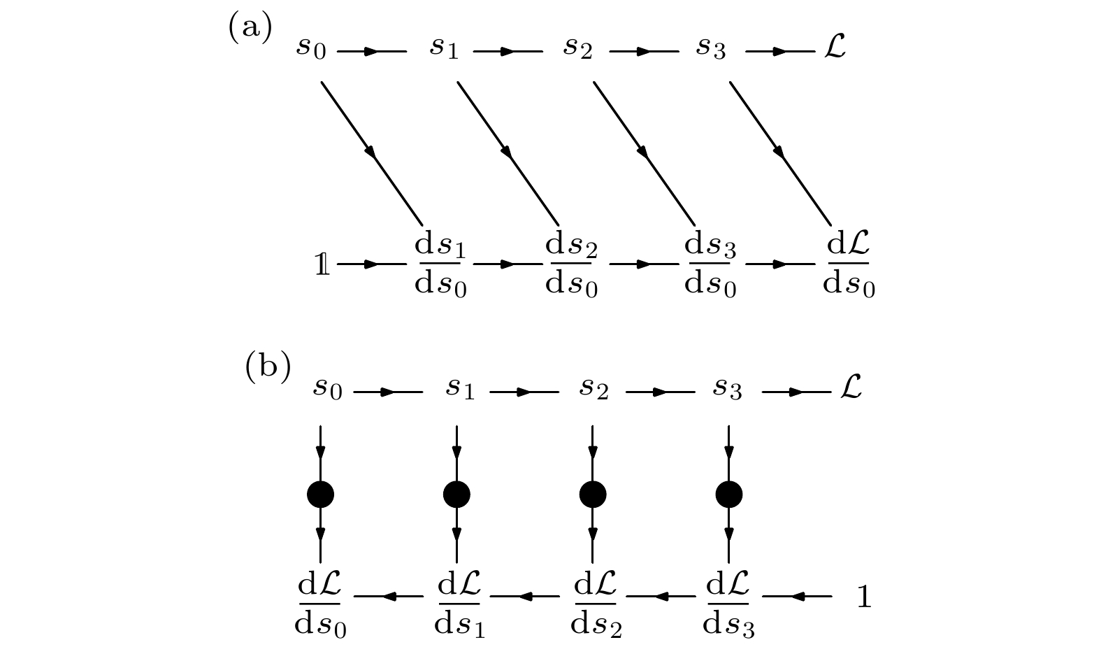
图 1 物理模拟程序中对状态变量梯度的(a)前向传播和(b)后向传播过程. 其中线条上的箭头代表运算的方向, 圆圈为后向自动微分中缓存的变量
Fig. 1. The (a) forward mode and (b) backward mode gradient propagation for state variables in a physics simulation. The arrows are computation directions, and circles are cached states in the backward mode automatic differentiation.

图 2 使用(a)检查点方案和(b)反计算方案避免缓存全部中间状态. 图中黑箭头为正常计算过程, 红箭头为梯度回传过程, 蓝箭头为梯度回传和反向计算的复合过程, 箭头上的数字代表了执行顺序. 黑色和白色的圆点为被缓存和未被缓存 (或通过反计算消除) 的状态
Fig. 2. Using (a) checkpointing scheme and (b) reverse computing scheme to avoid caching all intermediate states. The black arrows are regular forward computing, red arrows are gradient back propagation, and blue arrows are reverse computing. The numbers above the arrows are the execution order. Black and white circles represent cached states and not cached states (or those states deallocated in reverse computing) respecitively.
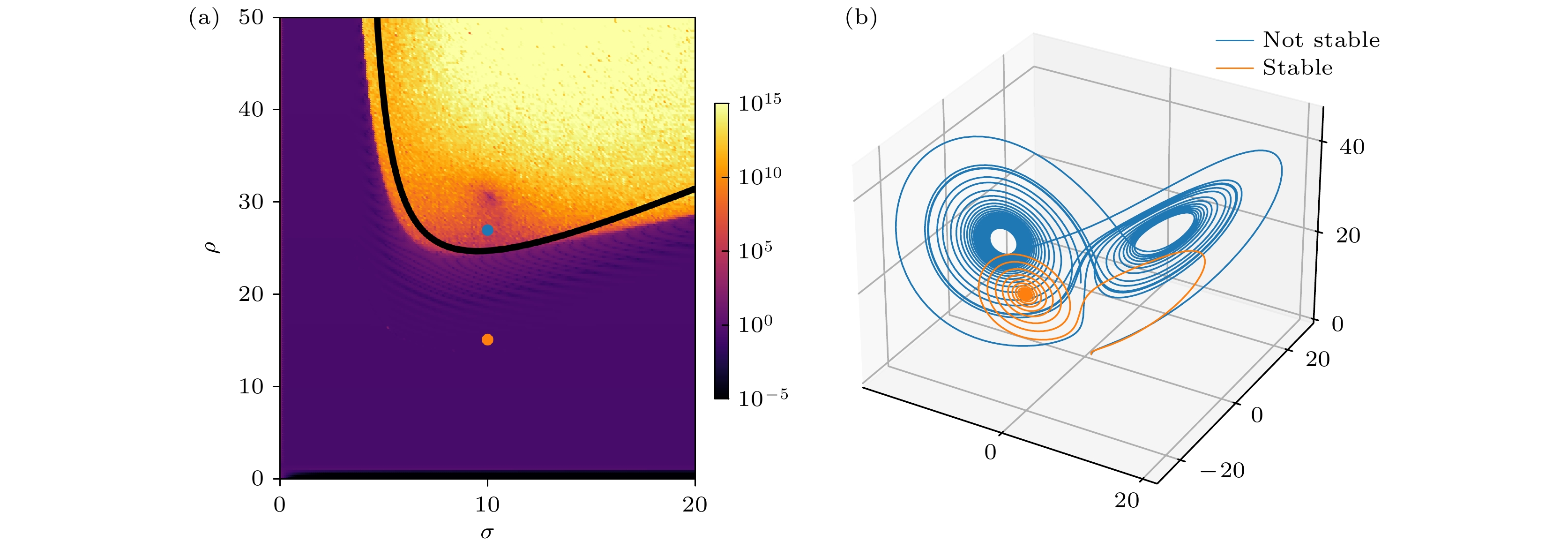
图 3 (a) 洛伦茨系统中固定参数
$\beta=8/3$ , 梯度大小与参数$\rho$ 和$\sigma$ 的关系. 图中颜色代表了平均梯度大小, 黑线是理论上会不会存在稳定吸引子分界线. (b) 中的蓝色和黄色的线分别对应 (a) 图标识的蓝点处参数$(\sigma=10, \rho=27)$ 和黄点处参数$(\sigma=10, \rho=15)$ 对应的动力学模拟Fig. 3. (a) The magnitude of gradients as a function of parameters
$\rho$ and$\sigma$ in a Lorenz system with$\beta$ fixed to$8/3$ . The black line is a theoretical predicted stable attractor phase transition line. The blue and yellow curves in (b) are simulations at parameters corresponding to the blue$(\sigma=10,\; \rho=27)$ and yellow$(\sigma=10,\; \rho=15)$ dots in (a).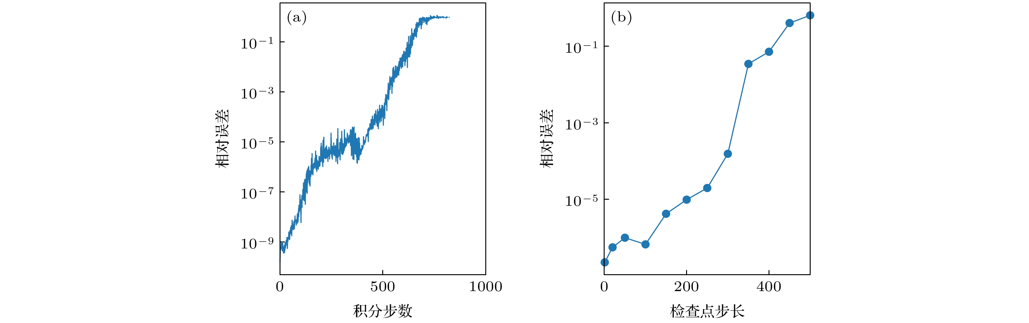
图 4 (a) 利用共轭态方法对
$\rho=27, \sigma=10, \beta=8/3$ 的洛伦茨系统求导时, 相对$l^2$ 误差与积分步数的关系. 其中一个点代表了在该步长下, 对$100$ 个随机初始点计算得到的中位数, 缺失的数据代表该处出现数值溢出. (b) 每隔固定步长设置检查点后,$10^4$ 步积分的误差Fig. 4. (a) Relative
$l^2$ error as a function of the integration step in differentiating the Lorenz equation solver at parameters$\rho=27,\; \sigma=10,\; \beta=8/3$ using the adjoint state method. Each data point in the graph represents a median of$100$ random samples. Some data are missing due to the numerical overflow. (b) The same error curve of computing$10^4$ steps with checkpointing to decrease the round off error.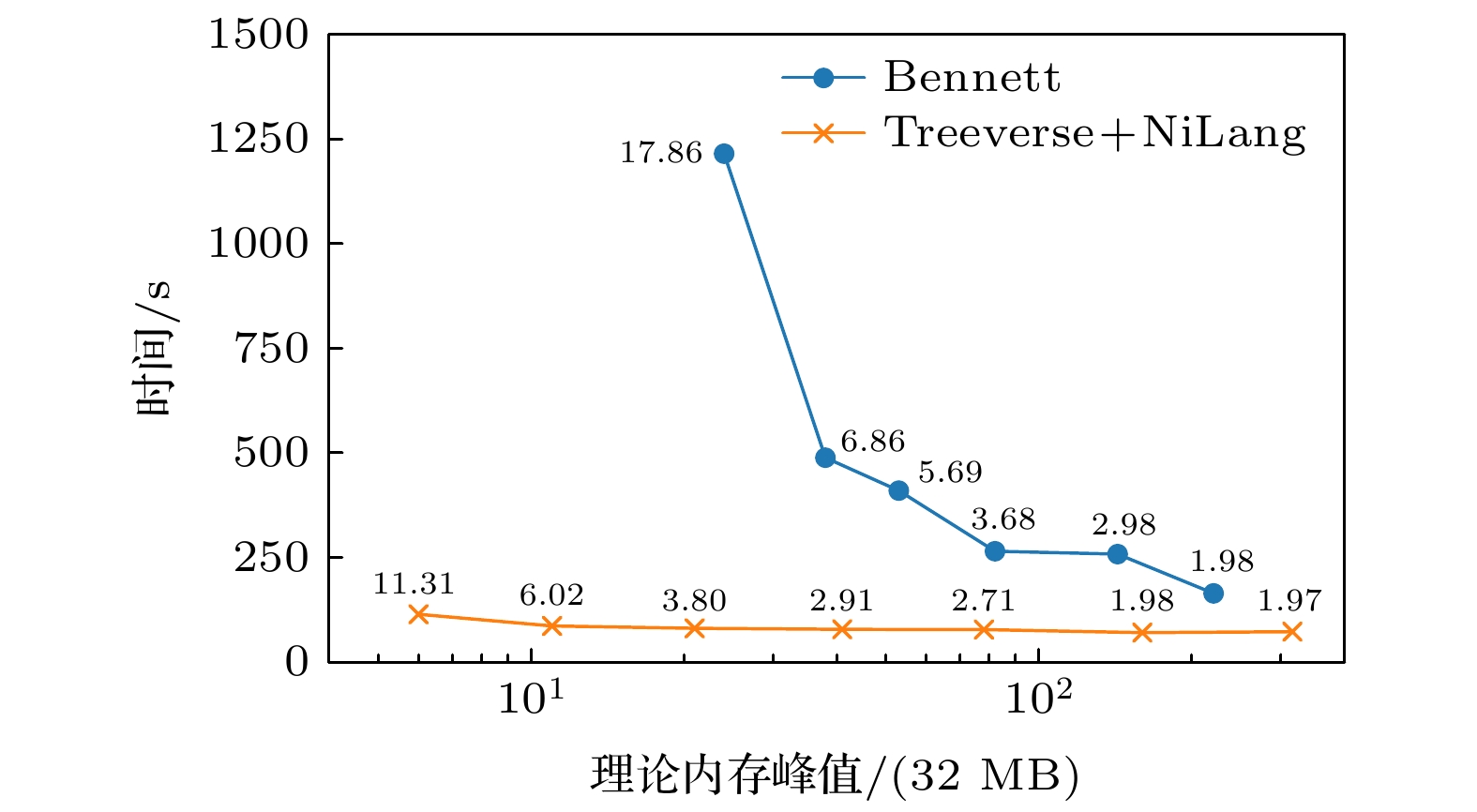
图 5 Bennett算法和Treeverse算法应用于PML求解过程的微分的时间与空间开销. 其中图中标记的数字为函数的实际前向运行步骤数与原始模拟步骤数 (
$10^4$ ) 的比值. 纵轴的总时间是前向计算和后向传播时间的总和, 横轴的空间的数值的实际含义为检查点的数目或可逆计算中的最大状态数. 在Bennett算法中, 后向运行次数和前向运行次数一样, 而Treeverse算法中, 反向传播的次数固定为$10^4$ Fig. 5. The time and space cost of using Bennett algorithm and Treeverse algorithm to solve the PML equation. The annotated numbers are relative forward overhead defined as the ratio between actual forward computing steps and the original computing steps. The time in the y axis is the actual time that includes both forward computing and back propagation. The space in the x axis is defined as the maximum number of checkpoints in the checkpointing scheme or the maximum intermediate states in the reverse computing scheme. In the Bennett's algorithm, the number of forward and backward steps are the same, while in Treeverse algorithm, the number of back propagation steps is fixed to
$10^4$ .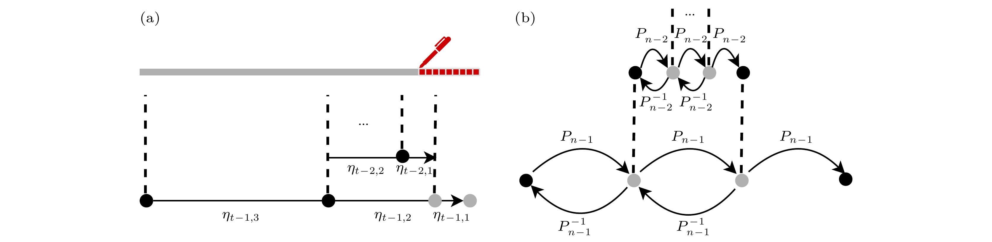
图 A1 (a) Treeverse算法[20]示意图, 其中
$\eta(\tau, \delta) \equiv \left(\begin{matrix} \tau + \delta \\ \delta \end{matrix}\right)=\dfrac{(\tau+\delta)!}{\tau!\delta!}$ ; (b) Bennett算法对应$k=3$ 的示意图[33,25], 其中P和$P^{-1}$ 分别代表了计算和反计算Fig. A1. (a) An illustration of the Treeverse algorithm[20], where
$\eta(\tau, \delta) \equiv \left(\begin{matrix} \tau + \delta \\ \delta \end{matrix}\right)=\dfrac{(\tau+\delta)!}{\tau!\delta!}$ . (b) An illustration of the Bennett's algorithm for$k=3$ [33,25], where P and$P^{-1}$ are forward computing and reverse computing respectively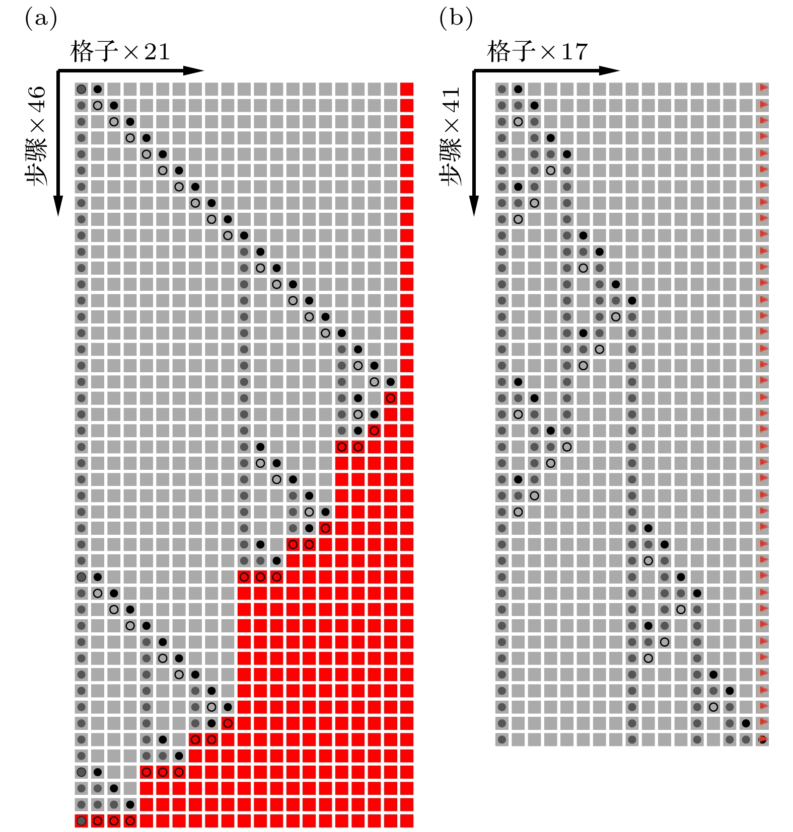
图 A2 (a) Treeverse算法 (
$\tau=3$ ,$\delta=3$ ) 和 (b) Bennett算法 ($k=2$ ,$n=4$ ) 对应的最优时间空间交换策略下的鹅卵石游戏解法, 横向是一维棋盘的格子, 纵向是步骤. 其中“○”为在这一步中收回的鹅卵石, “●”为在这一步中放上的鹅卵石, 而颜色稍淡的“ ”则对应之前步骤中遗留在棋盘上未收回的鹅卵石. (a) 中的红色格子代表已被涂鸦. (b) 中带旗帜的格点代表终点
Fig. A2. (a) The Treeverse algorithm(
$\tau=3 $ ,$\delta=3 $ ) and (b) Bennett's algorithm ($k=2 $ ,$n=4 $ ) solutions to the pebble game, the x direction is the grid layout and the y direction is the number of steps. Here, a “○” represents a pebble returned to the free pool in current step, a “●” represents the pebble added to the board in current step, and a “” represents a pebbles left on the board. In (a), red grids are painted grids. In (b), the grid with a flag sign is the goal.
图 A3 为了回溯中间状态, 时间和空间在两种最优时间-空间交换策略下的关系 (a) 固定横轴为状态回溯的计算时间与原函数计算时间的比值, 对比再允许固定时间开销下, 内存的额外开销. 其中Bennett算法代表了可逆计算下的最优策略, 而Treeverse则是传统计算允许的最优策略. (b) 对比Bennett算法与Treeverse算法空间开销的比值
Fig. A3. The time and space to trace back states in two time-space tradeoff strategies. (a) Space overheads versus time overheads at different numbers of simulation steps. The Bennett's algorithm is the optimal time-space tradeoff scheme in reversible computing, while the Treeverse algorithm is the optimal time-space tradeoff scheme in regular irreversible computing. (b) The ratio between the space overheads in the Bennett's algorithm and that in the Treeverse algorithm.
表 1 伴随状态法(算法1)
Table 1. Continuous adjoint state method (Algorithm 1)
输入: 动力学参数$\theta$, 开始时间$t_0$, 结束时间$t_n$, 末态$s_n$, 以及需要回传的导数$\dfrac{\partial {\cal{L} } }{\partial s_n}$ 输出: $\dfrac{\partial {\cal{L} } }{\partial s_0}$, $\dfrac{\partial {\cal{L} } }{\partial \theta}$ 1 function aug_dynamics((s, a, –), t, $\theta$) 2 $q=f(s, t, \theta)$ #定义拓展动力学函数 3 return $\left(q, \;-a^{\rm{T}}\dfrac{\partial q}{\partial s}\right.$, $\left. -a^{\rm{T}}\dfrac{\partial q}{\partial \theta}\right)$ 4 end 5 ${S_0} = \left( { {s_n}, \dfrac{ {\partial {\cal{L} } } }{ {\partial {s_n} } }, 0} \right)$ #计算拓展动力学函数的初始状态 6 $\left(s_0,\; \dfrac{\partial {\cal{L} } }{\partial s_0}\right.$, $\left.\dfrac{\partial {\cal{L} } }{\partial \theta}\right)$ = ODESolve(aug_dynamics, S0, $\theta$, $t_n$, t0) #对拓展动力学反向积分  下载: 导出CSV
表 2 不同自动微分方案中, 时间与空间复杂度的关系. 这里伴随状态法没有考虑了缓存部分中间结果以保证反向积分的正确性, 考虑之后应为
${\cal{O}}(TS)$ . 前向自动微分时间复杂度中的N代表了需要求导的参数个数. 可逆计算中的多项式时间复杂度中的$\epsilon > 0$ Table 2. The time and space complexities in different automatic differentiation schemes. Here, the adjoint state method does not consider the effect of round off error into consideration. The parameter N in the forward mode autodiff represent the number of differentiable input parameters. The
$\epsilon$ in the reverse computing is greater than 0.方法 时间 空间 是否严格 伴随状态法 ${\cal{O}}(T)$ ${\cal{O}}(S)$ 否 前向自动微分 ${\cal{O}}(NT)$ ${\cal{O}}(S)$ 是 基于最优检查点的
后向自动微分${\cal{O}}(T\log T)$ ${\cal{O}}(S\log T)$ 是 基于可逆计算的
后向自动微分${\cal{O}}(T^{1+\epsilon})$ ${\cal{O}}(S\log T)$ 是
下载: 导出CSV
表 3 不同方法对
$10^4$ 步洛伦茨系统积分过程的微分所需时间和空间, 其中空间部分以状态数目为单位, 时间的估计通过BenchmarkTools.jl软件包多次统计得出. 这里, NeuralODE中单步计算的微分由NiLang完成, 检查点的步长为200步Table 3. The time and space to simulate a
$10^4$ step Lorenz integration, where the space is measured in unit of single state size, and the time is obtained by repeated sample using the Julia package BenchmarkTools.jl. Here, the single step back propagation in NeuralODE is obtained with NiLang, and the checkpoint step size is 200.方法 Julia ForwardDiff NiLang Neural
ODE +
NiLang时间/ms 1.90 2.88 6.70 34.30 空间 (估计) 1 6 104 50
下载: 导出CSV
表 A1 鹅卵石游戏-可逆计算版本
Table A1. Pebble game rules—the reversible computing version
放置规则: 如果第$ i $个格子上有鹅卵石, 则可以从自己堆中 取一个鹅卵石放置于第$ i+1 $个格子中, 回收规则: 仅当第$ i $个格子上有鹅卵石, 才可以把第$ i+1 $ 个格子上的鹅卵石取下放入自己的堆中, 结束条件: 第$ n $个格子上有鹅卵石. 游戏目标: 在固定可使用鹅卵石数目为$ S $ (不包括初始鹅 卵石) 的前提下, 使用尽可能少的步骤数触发游 戏结束.
下载: 导出CSV
表 A2 Bennett算法
Table A2. The Bennett's algorithm
输入: 初始状态集合$S=\{0:s_0\}$, 子分块数目$k$, 分块 起点点$i=0$, 分块长度$L=n$ 输出: 末态$S[n]$ 1 function bennett (S, $k$, $i$, $L$) 2 if L = 1 then 3 $S[i+1]\leftarrow0$ 4 $S[i+1]+=f_iS[i]$ 5 else 6 $l\leftarrow\lceil {L}/{k} \rceil$ 7 $k'\leftarrow\lceil {L}/{l} \rceil$ 8 for $j=1,2,\cdots,k'$ do 9 bennett $(S, k, i+(j-1)l) $, min $(l,L(j-1) l))$ 10 end 11 for $j=k'-1,k'-2,\cdots 1$ do 12 bennett $(S, k, i+(j-1)l,l)$ 13 end 14 end 15 end
下载: 导出CSV
表 A3 鹅卵石游戏-检查点版本
Table A3. Pebble game rules—the checkpointing version
放置规则: 如果第$ i $个格子上有鹅卵石, 则可以从自己堆中取一个鹅卵石放置于第$ i+1 $个格子中. 回收规则: 可以随意把格子上的鹅卵石取下放入自己的堆中, 收回鹅卵石不计步骤数. 涂鸦规则: 当第$ i $个格子有鹅卵石, 且第$ i+1 $个格子被涂鸦, 可以涂鸦第$ i $个格子, 涂鸦不记入步骤数. 结束条件: 涂鸦完所有的格点. 游戏目标: 在固定可使用鹅卵石数目为$ S $ (不包括初始鹅卵石) 的前提下, 使用尽可能少的步骤数触发游戏结束.
下载: 导出CSV
表 A4 算法A2: Treeverse算法
Table A4. Algorithm A2: The Treeverse algorithm
输入: 状态缓存集合$S=\{0:s_0\}$, 需回传的梯度$\overline{s_n}\equiv $$ \dfrac{\partial {\cal{L} } }{\partial s_n}$, 允许缓存的状态数$\delta$, 扫描次数$\tau$, 分块起点$\beta=0$, 分开终点$\phi=n$内容 以及把分块分割为两部分的分割点$\sigma=0$ 输出: 回传的梯度$\overline{s_0} \equiv \dfrac{\partial {\cal{L} } }{\partial s_0}$ 1 function treeverse(S, $\overline{s_\phi}$, $\delta$, $\tau$, $\beta$, $\sigma$, $\phi$) 2 if $\sigma > \beta$ then 3 $\delta = \delta - 1$ 4 $s = S[\beta]$ #加载初始状态 $s_\beta$ 5 for $j=\beta, \beta+1, ..., \sigma-1$ do 6 $s_{j+1} = f_j(s_j)$ #计算$s_\sigma$ 7 end 8 $S[\sigma] = s_\sigma$ 9 end 10 #以$\kappa$为最优分割点(二项分布), 递归调用
Treeverse算法11 while $\tau>0$ and $\kappa={\rm{mid}}(\delta, \tau, \sigma, \phi) < \phi$ do 12 $\overline{s_{\kappa}}$ = treeverse(S, $\overline{s_\phi}$, $\delta$, $\tau$, $\sigma$, $\kappa$, $\phi$) 13 $\tau = \tau-1$ 14 $\phi = \kappa$ 15 end 16 $\overline{s_\sigma} \!=\! \overline{f_\sigma}(\overline{s_{\sigma+1} }, s_\sigma)$ #利用已有的$s_\sigma$和$\overline{s_\phi}$ 回
传导数17 if $\sigma>\beta$ then 18 remove($S[\sigma]$) # 从缓存的状态集合中移除$s_\sigma$ 19 end 20 return $\overline{s_\sigma}$ 21 end 22 function mid($\delta$, $\tau$, $\sigma$, $\phi$) #选取二项分布分割点 23 $\kappa = \lceil(\delta\sigma + \tau\phi)/(\tau+\delta)\rceil$ 24 if $\kappa \geq \phi$ and $\delta > 0$ then 25 $\kappa = \max(\sigma+1, \phi-1)$ 26 end 27 end
下载: 导出CSV
-
[1] Griewank A, Walther A 2008 SIAM, Evaluating derivatives: principles and techniques of algorithmic differentiation
[2] Rosset C 2019 Microsoft Blog, Turing-nlg: A 17-billion-parameter language model by microsoft
[3] Nolan J F 1953 Ph. D Dissertation (Cambridge: Massachusetts Institute of Technology)
[4] Wengert R E 1964 Communications of the ACM 7 463
Google Scholar
[5] Linnainmaa S 1976 BIT Numerical Mathematics 16 146
Google Scholar
[6] Gutzwiller M C 1963 Phys. Rev. Lett. 10 159
Google Scholar
[7] Carleo G and Troyer M 2017 Science 355 602
Google Scholar
[8] Deng D L, Li X P, Sarma S D 2017 Phys. Rev. X 7 021021
Google Scholar
[9] Cai Z, Liu J G 2018 Phys. Rev. B 97 035116
Google Scholar
[10] Luo X Z, Liu J G, Zhang P, Wang L 2020 Quantum 4 341
Google Scholar
[11] Liao H J, Liu J G, Wang L, Xiang T 2019 Phys. Rev. X 9 031041
Google Scholar
[12] Liu J G, Wang L, Zhang P 2021 Phys. Rev. Lett. 126 090506
Google Scholar
[13] Heimbach P, Hill C, Giering R 2005 Future Generation Computer Systems 21 1356
Google Scholar
[14] Symes W W 2007 Geographics 72 SM213
Google Scholar
[15] Zhu W Q, Xu K L, Darve E, Beroza G C 2021 Computers & Geosciences 151
Google Scholar
[16] Bradbury J, Frostig R, Hawkins P, Johnson M J, Leary C, Maclaurin D, Necula G, Paszke A, VanderPlas J, Wanderman-Milne S, Zhang Q 2018 Software, JAX: Composable Transformations of Python+NumPy Programs
[17] Paszke A, Gross S, Massa F, Lerer A, Bradbury J, Chanan G, Killeen T, Lin Z M, Gimelshein N, Antiga L, Desmaison A, Köpf A, Yang E, DeVito Z, Raison M, Tejani A, Chilamkurthy S, Steiner B, Fang L, Bai J J, Chintala S 2019 arXiv: 1912.01703
[18] Plessix R 2006 Geophysical Journal International 167 495
Google Scholar
[19] Chen R T, Rubanova Y, Bettencourt J, Duvenaud D K 2018 Advances in Neural Information Processing Systems Palais des Congrès de Montréal, Montréal, Canada
[20] Griewank A 1992 Optimization Methods and Software 1 35
Google Scholar
[21] Forget G, Campin J M, Heimbach P, Hill C N, Ponte R M, Wunsch C 2015 Geoscientific Model Development 8 3071
Google Scholar
[22] Hascoet L, Pascual V 2013 ACM Transactions on Mathematical Software (TOMS) 39 20
Google Scholar
[23] Utke J, Naumann U, Fagan M, Tallent N, Strout M, Heimbach P, Hill G, Wunsch C 2008 ACM Transactions on Mathematical Software (TOMS) 34 1
Google Scholar
[24] Liu J G, Zhao T 2020 arXiv: 2003.04617
[25] Levine R Y, Sherman A T 1990 SIAM Journal on Computing 19 673
Google Scholar
[26] Grote M J, Sim I 2010 arXiv 1001.0319
[27] Lorenz E N 1963 J. Atmospheric Sci. 20 130
Google Scholar
[28] Hirsch M W, Smale S, Devaney R L 2012 Differential Equations, Dynamical Systems, and An Introduction to Chaos (Cambridge: Academic Press)
[29] Revels J, Lubin M, Papamarkou R 2016 arXiv 1607.07892
[30] Berenger J P 1994 Journal of computational physics 114 185
Google Scholar
[31] Roden J A, Gedney S D 2000 Microwave Opt. Technol. Lett. 27 334
Google Scholar
[32] Martin R, Komatitsch D, Ezziani A 2008 Geophysics 73 T51
Google Scholar
[33] Bennett C H 1973 IBM journal of Research and Development 17 525
Google Scholar

 下载:
下载:


计量
- 文章访问数: 12598
- PDF下载量: 496
- 被引次数: 0
