


-
磁屏蔽在磁场敏感的装置如原子钟、原子干涉仪等精密设备中发挥重要的作用, 在变化外磁场下的某个磁屏蔽内部剩余磁场, 可以通过Jiles-Atherton磁滞模型和磁屏蔽系数计算得出, 根据计算结果可以进行主动补偿来抵消内部磁场的改变. 然而实际应用中磁滞模型中五个与磁屏蔽相关的参数以及磁场衰减的两个参数的准确值的获得是比较困难的, 通常根据实测磁滞回线人工匹配调节参数会花费大量时间且很难确保最终参数是全局最优值. 基于人工神经网络的机器学习方法已经成为一种对复杂模型进行参数优化的有效手段, 得益于现代计算机强大的运算能力, 该过程通常远远快于人工参数调节, 并有更大概率找到全局最优值, 获得优于手工调节的参数值. 本文利用人工神经网络在线机器学习的方法, 对磁滞模型的五个参数与磁屏蔽的另外两个屏蔽相关参数进行优化测定, 并对模拟卫星磁场环境下磁屏蔽内剩余磁场进行预测. 通过实际测量屏蔽筒内剩余磁场与预测值比对, 发现通过机器学习方法得到的磁屏蔽特性参数优于手动找到的参数, 且所用时间大大缩短. 该结果不仅有助于更好地进行磁场补偿, 用于冷原子系统参数优化调整, 更重要的是验证了神经网络在多参数物理系统中的应用, 可以使其他多参数共同作用的物理实验进行最优参数的快速确定.Magnetic shielding plays an important role in magnetically susceptible devices such as cold atom clocks, atomic interferometers and other precision equipment. The residual magnetic field in a magnetic shield under a varying external magnetic field can be calculated by the Jiles-Atherton (J-A) hysteresis model and magnetic shielding coefficient. According to the calculation results, the variation of internal magnetic field can be compensated for the active compensation coils. However, it is difficult to practically obtain the exact values of the five magnetic-shielding-related parameters in the J-A hysteresis model and the other two magnetic-field-attenuation-related parameters. It usually takes a lot of time to match the parameters manually according to the measured hysteresis loop and it is difficult to ensure that the final parameters are the global optimal values. The machine learning method based on artificial neural network has been used as an efficient method to optimize the parameters of complex systems. Owing to the powerful computing capability of modern computers, using the artificial neural network to optimize parameters is usually much faster than manual optimization method, and has a greater probability of finding the global optimal parameters. In this paper, the five J-A parameters and the other two parameters relating to magnetic field attenuation are optimized by the method of online learning based on artificial neural network, and the residual magnetic field in the magnetic shield is predicted under the simulated satellite magnetic field environment. By comparing the measured residual magnetic field with the predicted value, it is found that the machine learning method can optimize the magnetic shielding characteristic parameters more quickly and accurately than the manual optimization method. This result can not only help us to compensate for the magnetic field better and optimize the parameters of our cold atom system, but also validate the application of neural network in a multi-parameter physical system. This proves that the in-depth learning neural network can be conveniently applied to other physical experiments with multi-parameter interaction, and can quickly determine the optimal parameters needed in the experiment. This application is especially effective for remote experiments with slow response to parameter adjustment, such as scientific experiments carried out on satellites or deep space.
-
Keywords:
- artificial neural networks /
- magnetic shielding /
- hysteresis /
- cold atom clock
[1] Guéna J, Abgrall M, Rovera D, Laurent P H, Chupin B, Lours M, Santarelli G, Rosenbusch P, Tobar M E, Li R X, Gibble K, Clairon A, Bize S 2012 IEEE Trans. Ultra. Ferro. Freq. Cont. 59 391
 Google Scholar
[2] Ovchinnikov Y, Marra G 2011 Metrologia 48 87
Google Scholar
[3] Levi F, Calonico D, Calosso C E, Godone A, Micalizio S, Costanzo G A 2014 Metrologia 51 270
Google Scholar
[4] Gerginov V, Nemitz N, Weyers S, Schroder R, Griebsch D, Wynands R 2010 Metrologia 47 65
Google Scholar
[5] 王瑾, 詹明生 2018 物理学报 67 160402
Google Scholar
Wang J, Zhan M S 2018 Acta Phys. Sin. 67 160402
Google Scholar
[6] Moric I, Laurent P, Chatard P, de Graeve C M, Thomin S, Christophe V, Grosjean O 2014 Acta Astronaut. 102 287
Google Scholar
[7] Kubelka-Lange A, Herrmann S, Grosse J, Lämmerzahl C, Rasel E M, Braxmaier C 2016 Rev. Sci. Instrum. 87 063101
Google Scholar
[8] Morić I, de Graeve C M, Grosjean O, Laurent P 2014 Rev. Sci. Instrum. 85 075117
Google Scholar
[9] Li L, Ji J W, Ren W, Zhao X, Peng X K, Xiang J F, Lü D S, Liu L 2016 Chin. Phys. B 25 073201
Google Scholar
[10] Peng X K, Li L, Ren W, Ji J W, Xiang J F, Zhao J B, Ye M F, Zhao X, Wang B, Qu Q Z, Li T, Liu L, Lü D S 2019 AIP Adv. 9 035222
Google Scholar
[11] Liu L, Lü D S, Chen W B, Li T, Qu Q Z, Wang B, Li L, Ren W, Dong Z R, Zhao J B, Xia W B, Zhao X, Ji J W, Ye M F, Sun Y G, Yao Y Y, Song D, Liang Z G, Hu S J, Yu D H, Hou X, Shi W, Zang H G, Xiang J F, Peng X K, Wang Y Z 2018 Nat. Commun. 9 2760
Google Scholar
[12] Jiles D C, Atherton D L 1984 J. Appl. Phys. 55 2115
Google Scholar
[13] Jiles D C, Thoelke J B 1989 IEEE Trans. Magn. 25 3928
Google Scholar
[14] Jiles D C, Thoelke J B, Devine M K 1992 IEEE Trans. Magn. 28 27
Google Scholar
[15] Goodfellow I, Bengio Y, Courville A 2016 Deep Learning (Cambridge: MIT press) pp2-15
[16] Mnih V, Kavukcuoglu K, Silver D, Rusu A A, Veness J, Bellemare M G, Graves A, Riedmiller M, Fidjeland A K, Ostrovski G, Petersen S, Beattie C, Sadik A, Antonoglou I, King H, Kumaran D, Wierstra D, Legg S, Hassabis D 2015 Nature 518 529
Google Scholar
[17] Silver D, Huang A, Maddison C J, Guez A, Sifre L, Driessche G, Schrittwieser J, Antonoglou I, Panneershelvam V, Lanctot M, Dieleman S, Grewe D, Nham J, Kalchbrenner N, Sutskever I, Lillicrap T, Leach M, Kavukcuoglu K, Graepel T, Hassabis D 2016 Nature 529 484
Google Scholar
[18] Wigley P B, Everitt P J, van den Hengel A, Bastian J W, Sooriyabandara M A, McDonald G D, Hardman K S, Quinlivan C D, Manju P, Kuhn C C N, Petersen I R, Luiten A N, Hope J J, Robins N P, Hush M R 2016 Sci. Rep. 6 25890
Google Scholar
[19] Geisel I, Cordes K, Mahnke J, Jöllenbeck S, Ostermann J, Ertmer W, Klempt C 2013 Appl. Phys. Lett. 102 214105
Google Scholar
[20] Heinze G, Rudolf A, Beil F, Halfmann T 2010 Phys. Rev. A 81 053801
Google Scholar
[21] Palittapongarnpim P, Wittek P, Zahedinejad E, Vedaie S, Sanders B C 2017 Neurocomputing 268 116
Google Scholar
[22] Li C, de Celis Leal D R, Rana S, Gupta S, Sutti A, Greenhill S, Slezak T, Height M, Venkatesh S 2017 Sci. Rep. 7 5683
Google Scholar
[23] August M, Ni X 2017 Phys. Rev. A 95 012335
Google Scholar
[24] Ju S, Shiga T, Feng L, Hou Z, Tsuda K, Shiomi J 2017 Phys. Rev. X 7 021024
[25] Mavadia S, Frey V, Sastrawan J, Dona S, Biercuk M J 2017 Nat. Commun. 8 14106
Google Scholar
[26] Tranter A D, Slatyer H J, Hush M R, Leung A C, Everett J L, Paul K V, Vernaz-Gris P, Lam P K, Buchler B C, Campbell G T 2018 Nat. Commun. 9 4360
Google Scholar
[27] Li H Q, Li Q F, Xu X B, Lu T B, Zhang J J, Li L 2009 IEEE Trans. Magn. 47 1094
[28] 李慧奇, 杨延菊, 邓聘 2012 电网与清洁能源 28 19
Google Scholar
Li H Q, Yang Y J, Deng P 2012 Power System and Clean Energy 28 19
Google Scholar
[29] Araneo R, Celozzi S 2003 IEEE Trans. Magn. 39 1046
Google Scholar
[30] Bergqvist A J 1996 IEEE Trans. Magn. 32 4213
Google Scholar
[31] Bastos J P A, Sadowski N 2003 Electromagnetic Modeling by Finite Element Methods (Boca Raton: CRC press) pp250-275
[32] Hush M R, Slatyer H 2017 https://github.com/charmasaur/M-LOOP [2019-2-22]
[33] Byrd R H, Lu P H, Nocedal J, Zhu C 1995 SIAM J. Sci. Comput. 16 1190
Google Scholar
[34] Abadi M, Agarwal A, Barham P, Brevdo E, Chen Z, Citro C, Ghemawat S 2015 tensorflow.org[2019-2-22]
[35] Hart R A, Xu X, Legere R, Gibble K 2007 Nature 446 892
Google Scholar
[36] Wang B, Lü D S, Qu Q Z, Zhao J B, Li T, Liu L, Wang Y Z 2011 Chin. Phys. Lett. 28 63701
Google Scholar
-
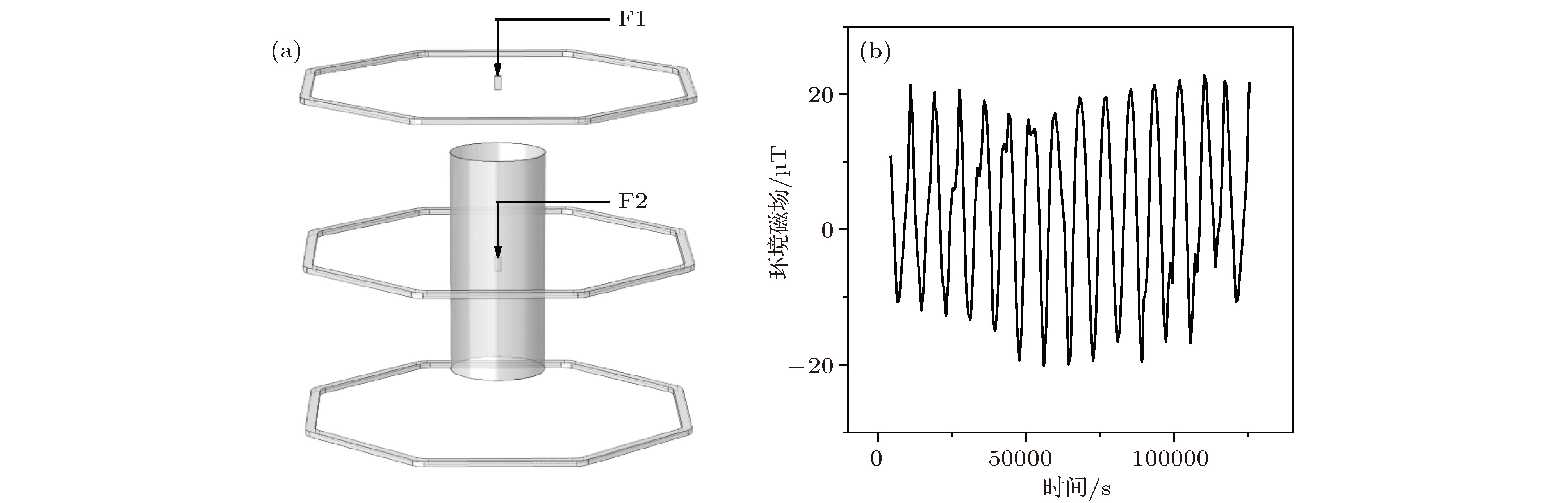
图 1 (a)实验装置示意图, 同时也是有限元仿真时所用的模型图; (b)对模型进行测试所用的近地轨道环境磁场
Fig. 1. (a) The schematic diagram of the experimental device and also the model diagram used in our finite element simulation; (b) low Earth orbit environmental magnetic field used to test the model.
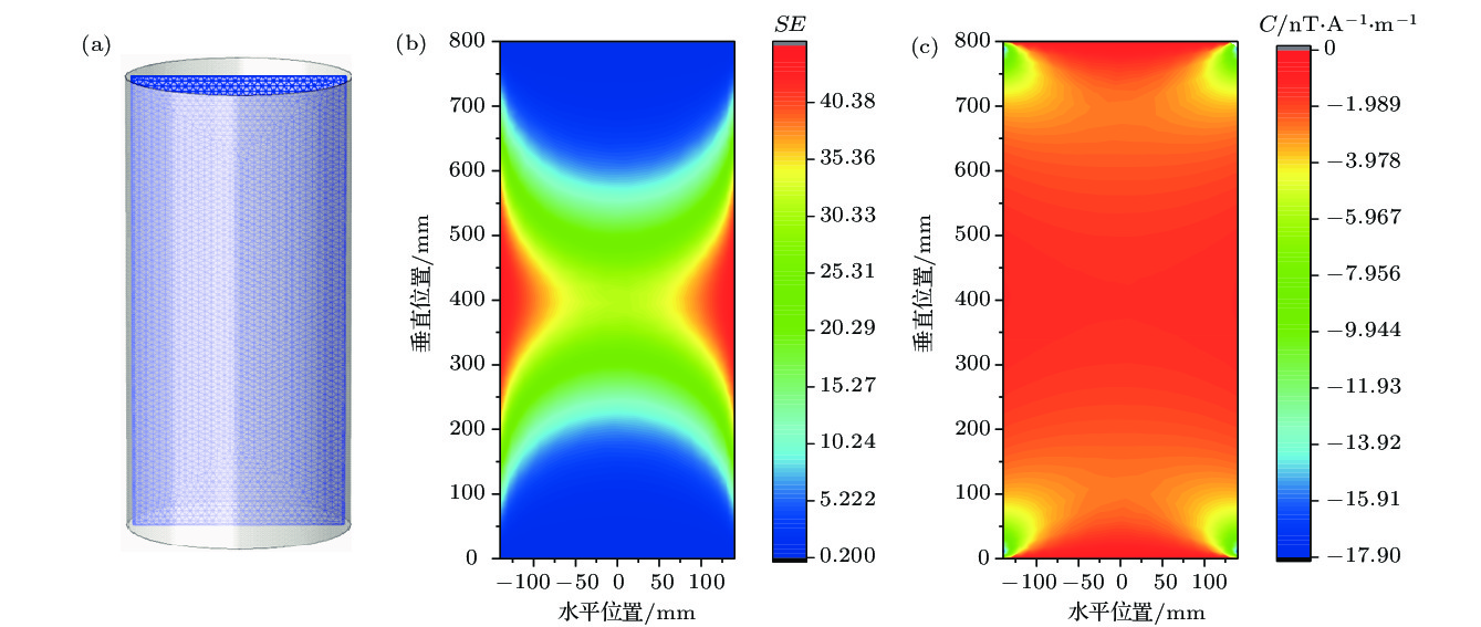
图 2 (a)数据所在磁屏蔽筒截面示意图; (b)有限元仿真所得到屏蔽内一个截面上的屏蔽效率分布图; (c)有限元仿真得到的屏蔽内一个截面上的磁化强度比例系数图
Fig. 2. (a) A schematic view of the section of the data; (b) the shielding efficiency distribution on a section inside the shield calculated by FEM software; (c) the magnetization intensity ratio coefficient on a section of the shield calculated by FEM software.

图 3 神经网络调参原理示意图 使用2个隐藏层的全连接神经网络, 每层32个神经元, 一旦神经网络训练完成, 就能调用scipy库预测最优参数
Fig. 3. Principle of optimizing with neural network. We use 2 hidden layers of full connected neural network, 32 neurons per layer. Once the neural network training is completed, we can use scipy to predict the optimal parameters
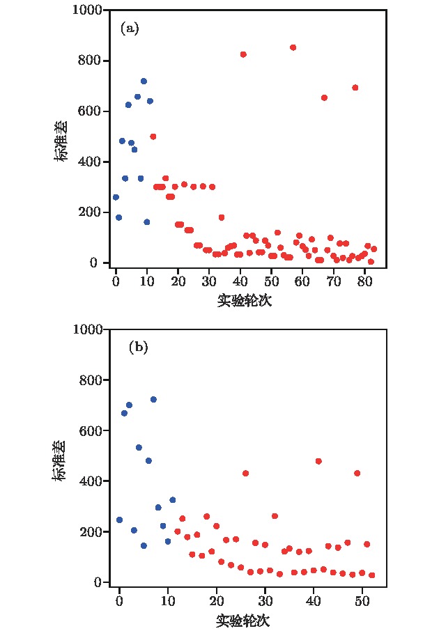
图 4 (a)当选用2层网络各32个神经元时, 预测标准差收敛性好且最小值仅为4.9; (b)当选用3层网络各64个神经元时, 由于过拟合预测标准差振荡且最小值为27
Fig. 4. (a) When 32 neurons of the 2 layers network are selected, the convergence of the prediction standard deviation is good and the minimum value is only 4.9; (b) when 64 neurons of the 3 layers network are selected, the convergence of the prediction standard deviation is poor because of over-fit and the minimum value is 27.

图 5 自动调参的流程图
Fig. 5. The flow chart of optimizing magnetic shielding characteristic parameters.
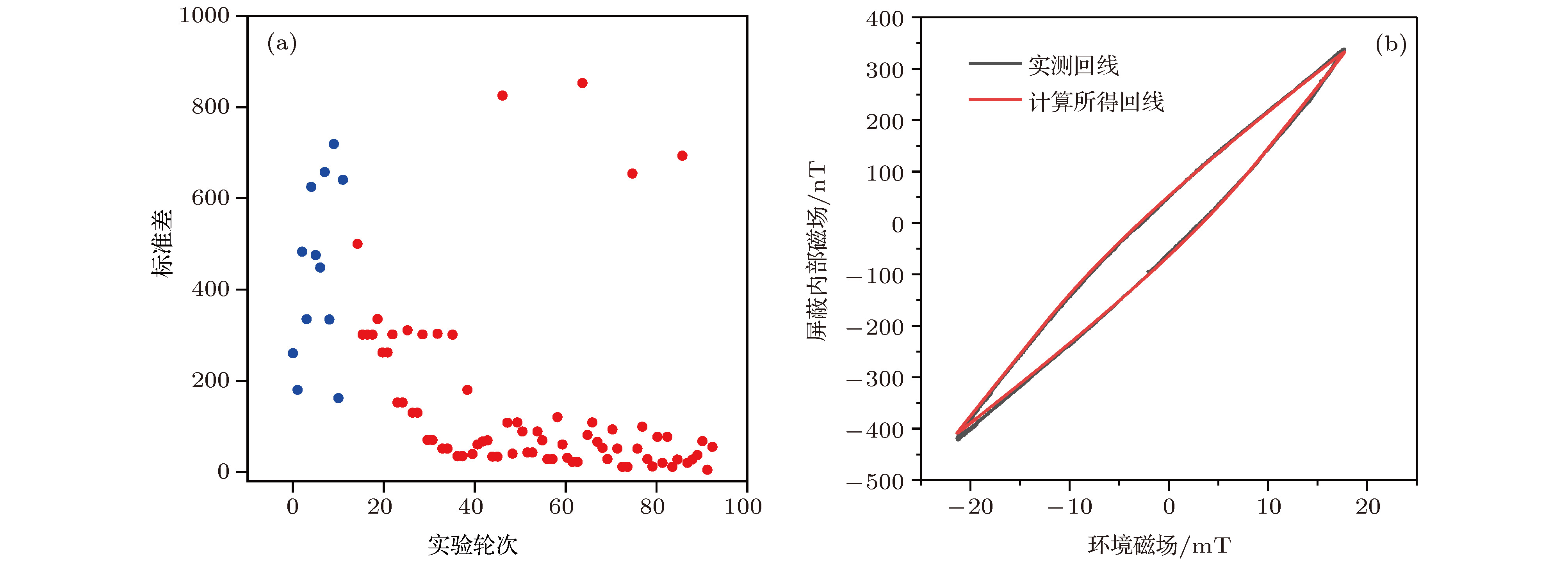
图 6 (a)一个典型的求参过程图, 预测参数值的标准差随实验轮次逐渐降低; (b)相应参数计算得到的磁滞回线与实测回线的比较
Fig. 6. (a) A typical continuation process graph, the standard deviation of the predicted parameter values is gradually reduced with the experimental round; (b) comparison of hysteresis loop and measured loop calculated by corresponding parameters.
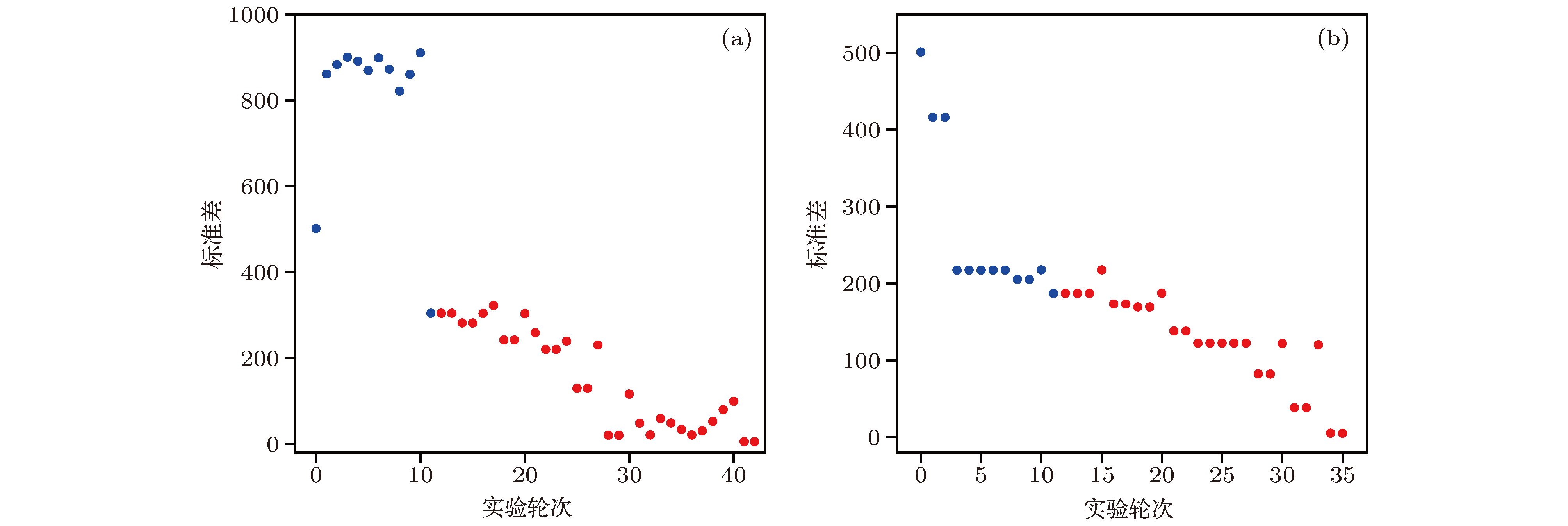
图 7 另外两组不同随机初始训练参数下, 标准差随实验轮次的收敛图
Fig. 7. Convergence graph of standard deviation with experimental rounds under two different random initial training parameters.
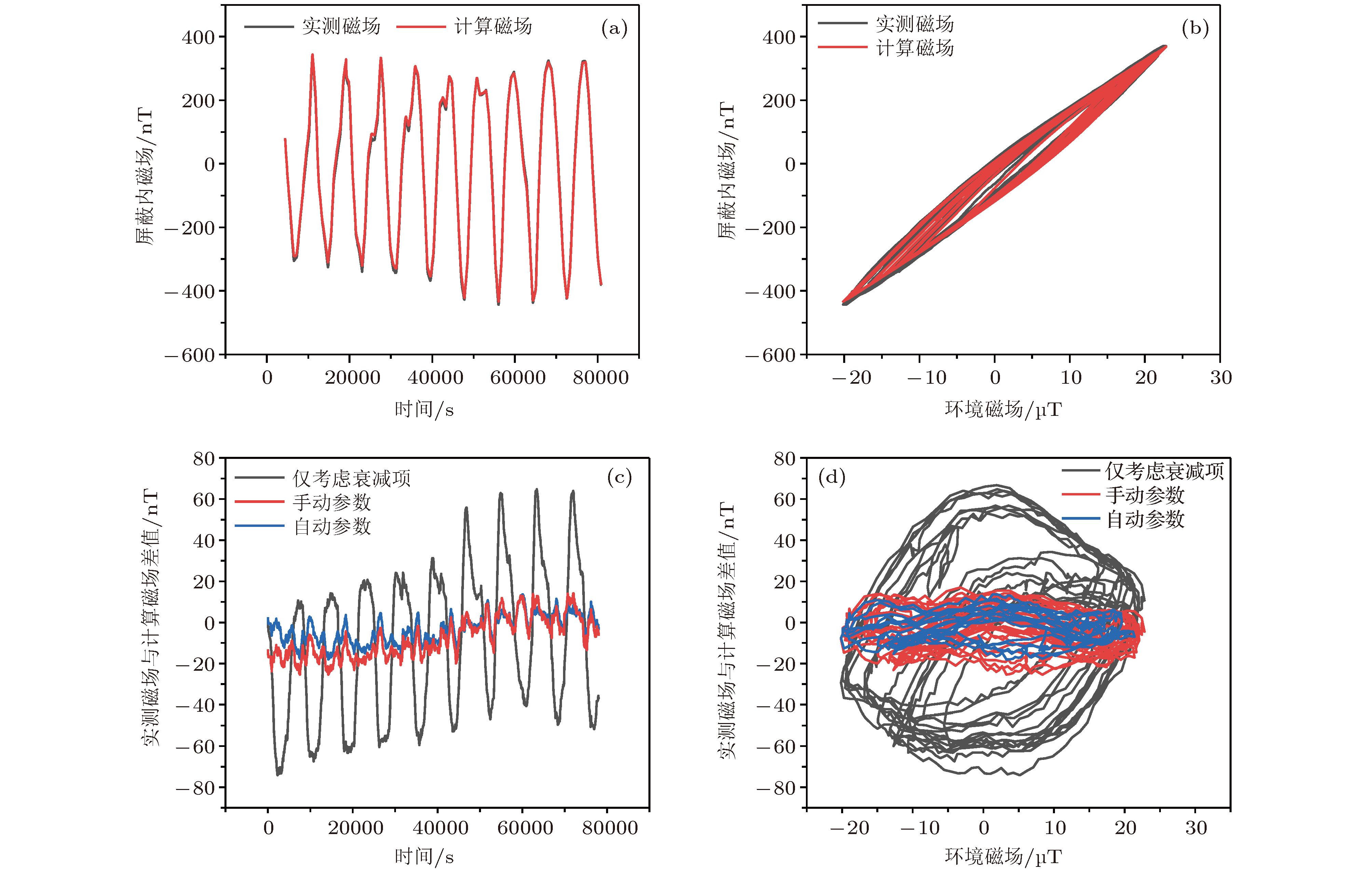
图 8 在近地轨道磁场环境下实测磁场与计算磁场的对比图 (a)横坐标为时间; (b)横坐标为环境磁场; (c) 使用手动调节参数, 自动求得的参数, 以及仅考虑衰减项不考虑磁化项, 计算磁场与实测磁场的差值, 横坐标为时间; (d)横坐标为环境磁场
Fig. 8. A comparison of the measured magnetic field with the calculated magnetic field in a near-Earth orbit magnetic field environment; (a) The x axis is time; (b) the x-axis is the ambient magnetic field; (c) use manual adjustment parameters, automatically obtained parameters, and simple
$ {B_{SE}}$ to calculate the difference between the magnetic field and the measured magnetic field, the abscissa is time; (d) the x-axis is the ambient magnetic field.表 1 手动调参和自动调参得到的参数值
Table 1. Parameter values obtained by manual tuning and automatic tuning.
参数名称 手动参数 自动参数 Ms 540000 540074 a 19555 19817 k 8.0 9.50 α 0 0 c 0.2 0.58 SE 31 36.37 C –1.8 –2.37  下载: 导出CSV
-
[1] Guéna J, Abgrall M, Rovera D, Laurent P H, Chupin B, Lours M, Santarelli G, Rosenbusch P, Tobar M E, Li R X, Gibble K, Clairon A, Bize S 2012 IEEE Trans. Ultra. Ferro. Freq. Cont. 59 391
Google Scholar
[2] Ovchinnikov Y, Marra G 2011 Metrologia 48 87
Google Scholar
[3] Levi F, Calonico D, Calosso C E, Godone A, Micalizio S, Costanzo G A 2014 Metrologia 51 270
Google Scholar
[4] Gerginov V, Nemitz N, Weyers S, Schroder R, Griebsch D, Wynands R 2010 Metrologia 47 65
Google Scholar
[5] 王瑾, 詹明生 2018 物理学报 67 160402
Google Scholar
Wang J, Zhan M S 2018 Acta Phys. Sin. 67 160402
Google Scholar
[6] Moric I, Laurent P, Chatard P, de Graeve C M, Thomin S, Christophe V, Grosjean O 2014 Acta Astronaut. 102 287
Google Scholar
[7] Kubelka-Lange A, Herrmann S, Grosse J, Lämmerzahl C, Rasel E M, Braxmaier C 2016 Rev. Sci. Instrum. 87 063101
Google Scholar
[8] Morić I, de Graeve C M, Grosjean O, Laurent P 2014 Rev. Sci. Instrum. 85 075117
Google Scholar
[9] Li L, Ji J W, Ren W, Zhao X, Peng X K, Xiang J F, Lü D S, Liu L 2016 Chin. Phys. B 25 073201
Google Scholar
[10] Peng X K, Li L, Ren W, Ji J W, Xiang J F, Zhao J B, Ye M F, Zhao X, Wang B, Qu Q Z, Li T, Liu L, Lü D S 2019 AIP Adv. 9 035222
Google Scholar
[11] Liu L, Lü D S, Chen W B, Li T, Qu Q Z, Wang B, Li L, Ren W, Dong Z R, Zhao J B, Xia W B, Zhao X, Ji J W, Ye M F, Sun Y G, Yao Y Y, Song D, Liang Z G, Hu S J, Yu D H, Hou X, Shi W, Zang H G, Xiang J F, Peng X K, Wang Y Z 2018 Nat. Commun. 9 2760
Google Scholar
[12] Jiles D C, Atherton D L 1984 J. Appl. Phys. 55 2115
Google Scholar
[13] Jiles D C, Thoelke J B 1989 IEEE Trans. Magn. 25 3928
Google Scholar
[14] Jiles D C, Thoelke J B, Devine M K 1992 IEEE Trans. Magn. 28 27
Google Scholar
[15] Goodfellow I, Bengio Y, Courville A 2016 Deep Learning (Cambridge: MIT press) pp2-15
[16] Mnih V, Kavukcuoglu K, Silver D, Rusu A A, Veness J, Bellemare M G, Graves A, Riedmiller M, Fidjeland A K, Ostrovski G, Petersen S, Beattie C, Sadik A, Antonoglou I, King H, Kumaran D, Wierstra D, Legg S, Hassabis D 2015 Nature 518 529
Google Scholar
[17] Silver D, Huang A, Maddison C J, Guez A, Sifre L, Driessche G, Schrittwieser J, Antonoglou I, Panneershelvam V, Lanctot M, Dieleman S, Grewe D, Nham J, Kalchbrenner N, Sutskever I, Lillicrap T, Leach M, Kavukcuoglu K, Graepel T, Hassabis D 2016 Nature 529 484
Google Scholar
[18] Wigley P B, Everitt P J, van den Hengel A, Bastian J W, Sooriyabandara M A, McDonald G D, Hardman K S, Quinlivan C D, Manju P, Kuhn C C N, Petersen I R, Luiten A N, Hope J J, Robins N P, Hush M R 2016 Sci. Rep. 6 25890
Google Scholar
[19] Geisel I, Cordes K, Mahnke J, Jöllenbeck S, Ostermann J, Ertmer W, Klempt C 2013 Appl. Phys. Lett. 102 214105
Google Scholar
[20] Heinze G, Rudolf A, Beil F, Halfmann T 2010 Phys. Rev. A 81 053801
Google Scholar
[21] Palittapongarnpim P, Wittek P, Zahedinejad E, Vedaie S, Sanders B C 2017 Neurocomputing 268 116
Google Scholar
[22] Li C, de Celis Leal D R, Rana S, Gupta S, Sutti A, Greenhill S, Slezak T, Height M, Venkatesh S 2017 Sci. Rep. 7 5683
Google Scholar
[23] August M, Ni X 2017 Phys. Rev. A 95 012335
Google Scholar
[24] Ju S, Shiga T, Feng L, Hou Z, Tsuda K, Shiomi J 2017 Phys. Rev. X 7 021024
[25] Mavadia S, Frey V, Sastrawan J, Dona S, Biercuk M J 2017 Nat. Commun. 8 14106
Google Scholar
[26] Tranter A D, Slatyer H J, Hush M R, Leung A C, Everett J L, Paul K V, Vernaz-Gris P, Lam P K, Buchler B C, Campbell G T 2018 Nat. Commun. 9 4360
Google Scholar
[27] Li H Q, Li Q F, Xu X B, Lu T B, Zhang J J, Li L 2009 IEEE Trans. Magn. 47 1094
[28] 李慧奇, 杨延菊, 邓聘 2012 电网与清洁能源 28 19
Google Scholar
Li H Q, Yang Y J, Deng P 2012 Power System and Clean Energy 28 19
Google Scholar
[29] Araneo R, Celozzi S 2003 IEEE Trans. Magn. 39 1046
Google Scholar
[30] Bergqvist A J 1996 IEEE Trans. Magn. 32 4213
Google Scholar
[31] Bastos J P A, Sadowski N 2003 Electromagnetic Modeling by Finite Element Methods (Boca Raton: CRC press) pp250-275
[32] Hush M R, Slatyer H 2017 https://github.com/charmasaur/M-LOOP [2019-2-22]
[33] Byrd R H, Lu P H, Nocedal J, Zhu C 1995 SIAM J. Sci. Comput. 16 1190
Google Scholar
[34] Abadi M, Agarwal A, Barham P, Brevdo E, Chen Z, Citro C, Ghemawat S 2015 tensorflow.org[2019-2-22]
[35] Hart R A, Xu X, Legere R, Gibble K 2007 Nature 446 892
Google Scholar
[36] Wang B, Lü D S, Qu Q Z, Zhao J B, Li T, Liu L, Wang Y Z 2011 Chin. Phys. Lett. 28 63701
Google Scholar

 下载:
下载:

计量
- 文章访问数: 18342
- PDF下载量: 170
- 被引次数: 0
