


-
随着深度学习处理问题的日益复杂, 神经网络的层数、神经元个数、和神经元之间的连接逐渐增加, 参数规模急剧膨胀, 优化超参数来提高神经网络的预测性能成为一个重要的任务. 文献中寻找最优参数的方法如灵敏度剪枝、网格搜索等, 算法复杂而且计算量庞大. 本文提出一种超参数优化的“删除垃圾神经元策略”. 权重矩阵中权重均值小的神经元, 在预测中的贡献可以忽略, 称为垃圾神经元. 该策略就是通过删除这些垃圾神经元得到精简的网络结构, 来有效缩短计算时间, 同时提高预测准确率和模型泛化能力. 采用这一策略, 长短期记忆网络模型对几种典型混沌动力系统的预测性能得到显著改善.With the complexity of problems in reality increasing, the sizes of deep learning neural networks, including the number of layers, neurons, and connections, are increasing in an explosive way. Optimizing hyperparameters to improve the prediction performance of neural networks has become an important task. In literatures, the methods of finding optimal parameters, such as sensitivity pruning and grid search, are complicated and cost a large amount of computation time. In this paper, a hyperparameter optimization strategy called junk neuron deletion is proposed. A neuron with small mean weight in the weight matrix can be ignored in the prediction, and is defined subsequently as a junk neuron. This strategy is to obtain a simplified network structure by deleting the junk neurons, to effectively shorten the computation time and improve the prediction accuracy and model the generalization capability. The LSTM model is used to train the time series data generated by Logistic, Henon and Rossler dynamical systems, and the relatively optimal parameter combination is obtained by grid search with a certain step length. The partial weight matrix that can influence the model output is extracted under this parameter combination, and the neurons with smaller mean weights are eliminated with different thresholds. It is found that using the weighted mean value of 0.1 as the threshold, the identification and deletion of junk neurons can significantly improve the prediction efficiency. Increasing the threshold accuracy will gradually fall back to the initial level, but with the same prediction effect, more operating costs will be saved. Further reduction will result in prediction ability lower than the initial level due to lack of fitting. Using this strategy, the prediction performance of LSTM model for several typical chaotic dynamical systems is improved significantly.
-
Keywords:
- LSTM /
- chaotic time series prediction /
- hyperparameter optimization /
- junk neuron deletion strategy
[1] 邓帅 2019 计算机应用研究 36 1984
Deng S 2019 Appl. Res. Comput. 36 1984
[2] 邵恩泽, 吴正勇, 王灿 2020 工业控制计算机 33 11
 Google Scholar
Shao E Z, Wu Z Y, Wang C 2020 Ind. Contrl. Comput. 33 11
Google Scholar
[3] 乔俊飞, 樊瑞元, 韩红桂, 阮晓钢 2010 控制理论与应用 27 111
Qiao J F, Fan R Y, Han H G, Ruan X G 2010 Contl. Theor. Appl. 27 111
[4] 陈国茗, 于腾腾, 刘新为 2021 数值计算与计算机应用 42 215
Google Scholar
Chen G M, Yu T T, Liu X W 2021 J. Num. Method. Comp. Appl. 42 215
Google Scholar
[5] 魏德志, 陈福集, 郑小雪 2015 物理学报 64 110503
Google Scholar
Wei D Z, Chen F J, Zheng X X 2015 Acta Phys. Sin. 64 110503
Google Scholar
[6] 王新迎, 韩敏 2015 物理学报 64 070504
Google Scholar
Wang X Y, Han M 2015 Acta Phys. Sin 64 070504
Google Scholar
[7] 黄伟建, 李永涛, 黄远 2021 物理学报 70 010501
Google Scholar
Huang W J, Li Y T, Huang Y 2021 Acta Phys. Sin. 70 010501
Google Scholar
[8] Yamaguti Y, Tsuda I 2021 Chaos 31 013137
Google Scholar
[9] Graves A 2013 arXiv: 1308.0850 [cs. NE]
[10] Johnston D E 1978 Proc 8 th BHRA Int Conf Fluid Sealing Durham, UK, 1978 pC1-1
[11] Sezer O B, Gudelek M U, Ozbayoglu A M 2020 Appl. Soft Comput. J. 90 106181
Google Scholar
[12] 甘文娟, 陈永红, 韩静, 王亚飞 2020 计算机系统应用 29 212
Google Scholar
Gan W J, Chen Y H, Han J, Wang Y F 2020 Comput. Syst. Appl. 29 212
Google Scholar
[13] Farmelo G 2002 It Must Be Beautiful: Great Equations of Modern Science (London: Granta Publications) pp28–45
[14] Grassberger P, Procaccia I 1983 Physica D 9 189
Google Scholar
[15] Nauenberg M 1983 Ann. N. Y. Acad. Sci. 410 317
Google Scholar
[16] 张中华, 丁华福 2009 计算机技术与发展 19 185
Google Scholar
Zhang Z H, Ding H F 2009 Comput. Technol. Dev. 19 185
Google Scholar
[17] Butcher J C 1967 J. ACM 14 84
Google Scholar
[18] Liu C, Yin S Q, Zhang M, Zeng Y, Liu J Y 2014 Appl. Mech. Mater. 644-650 2216
[19] Bao Y K, Liu Z T 2006 LNCS 4224 504
[20] Ou Y Y, Chen G H, Oyang Y J 2006 LNCS 4099 1017
-
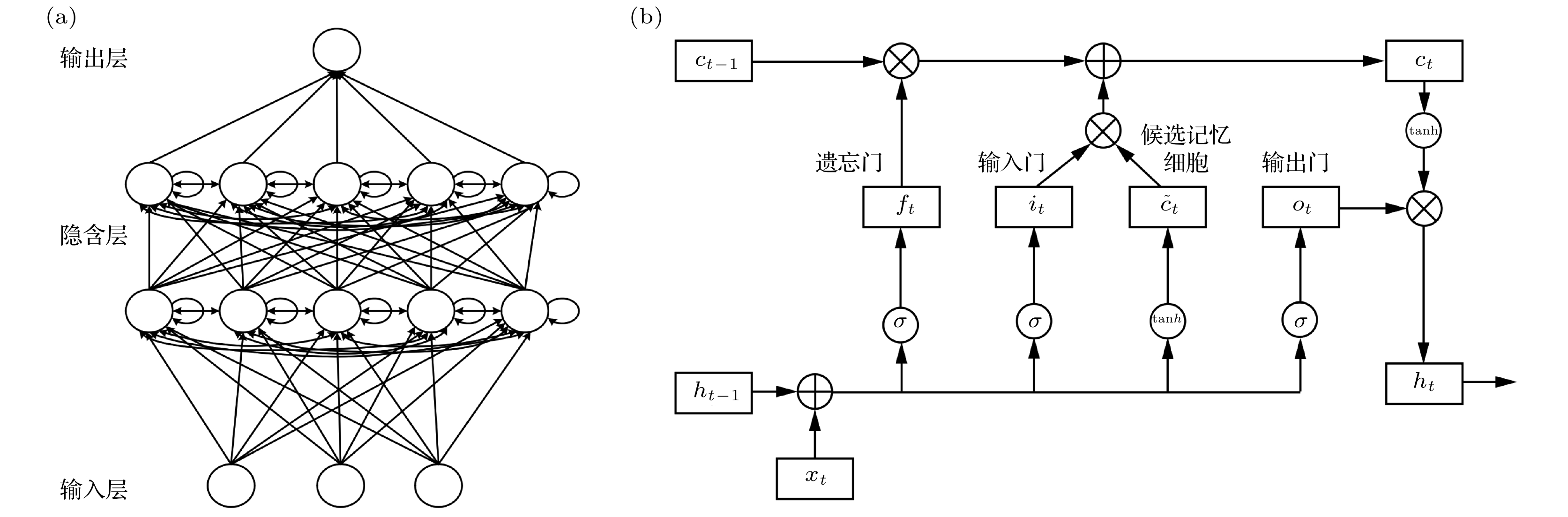
图 1 LSTM神经网络 (a) LSTM模型网络结构; (b)单元内部运行逻辑
Fig. 1. LSTM neural network: (a) network structure of LSTM; (b) run logic inside the cell.
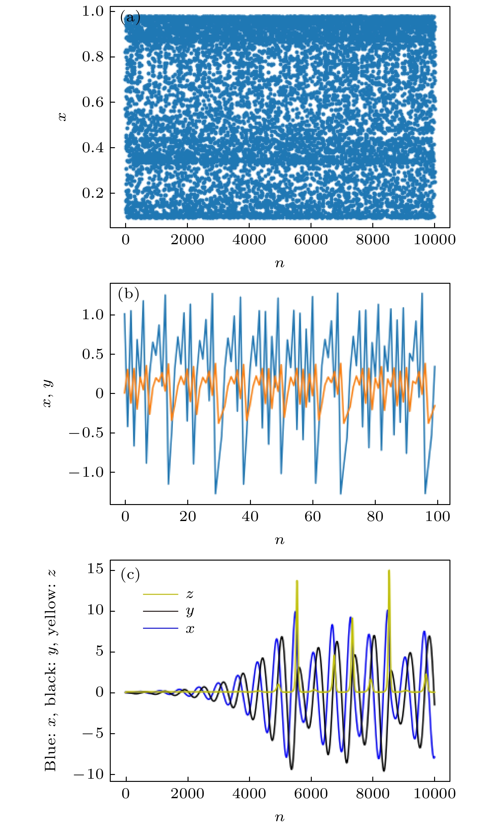
图 2 混沌时间序列 (a) Logistic系统, μ
$ =3.9 $ ; (b) Henon系统; (c) Rossler系统Fig. 2. Chaotic time series: (a) Logistic system, μ
$ =3.9 $ ; (b) Henon system; (c) Rossler system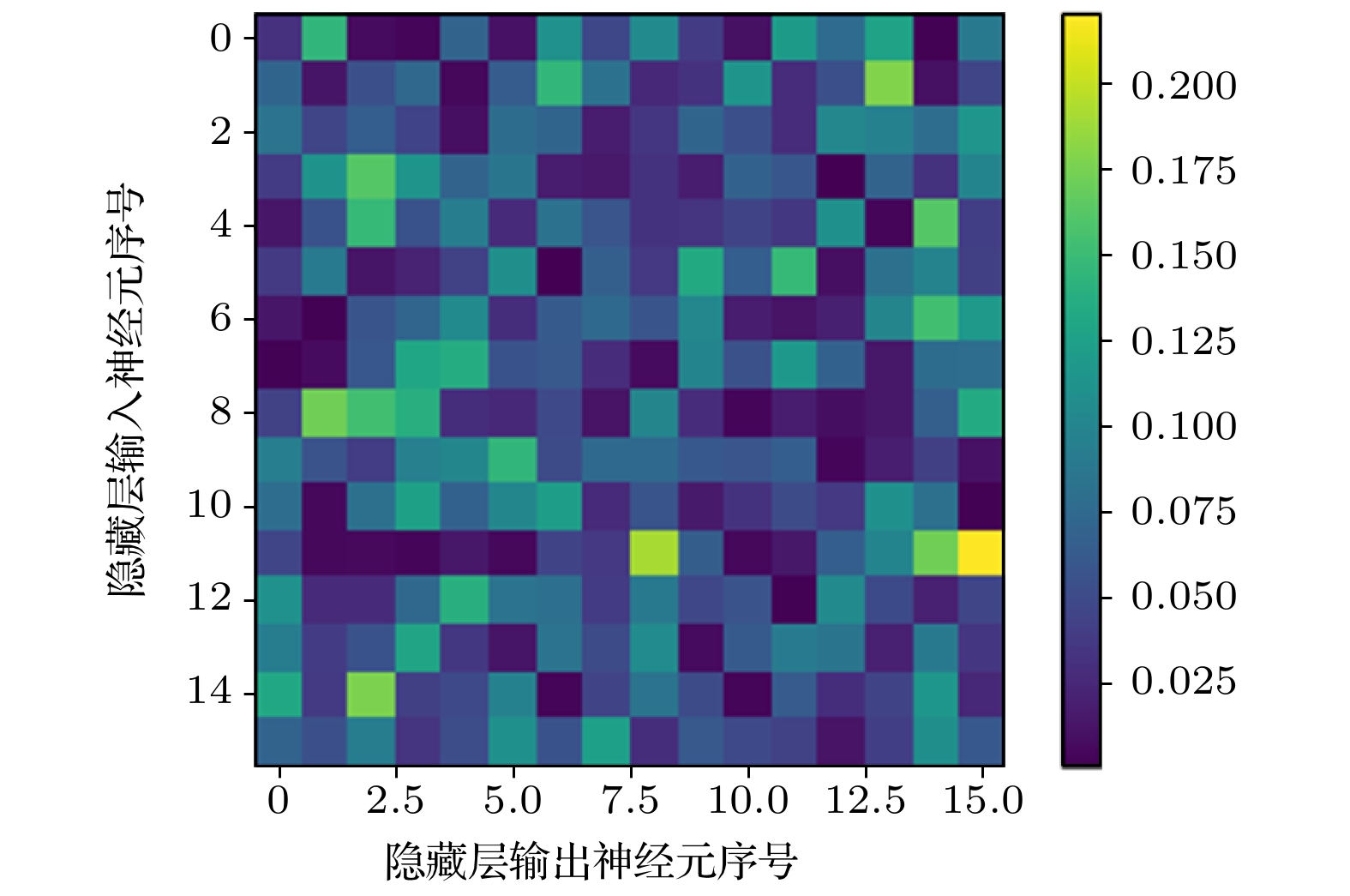
图 3 隐藏层输入神经元对输出神经元的权重热图
Fig. 3. Heat map of weight of input neuron to output neuron in hidden layer.
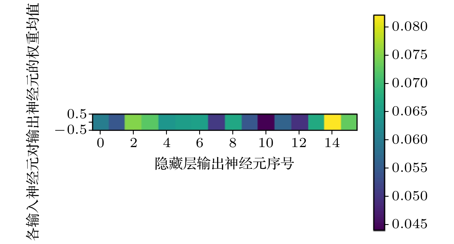
图 4 隐藏层各输入神经元对输出神经元的权重均值热图
Fig. 4. Heat map of weights’ mean value of input neurons to output neurons in hidden layer.
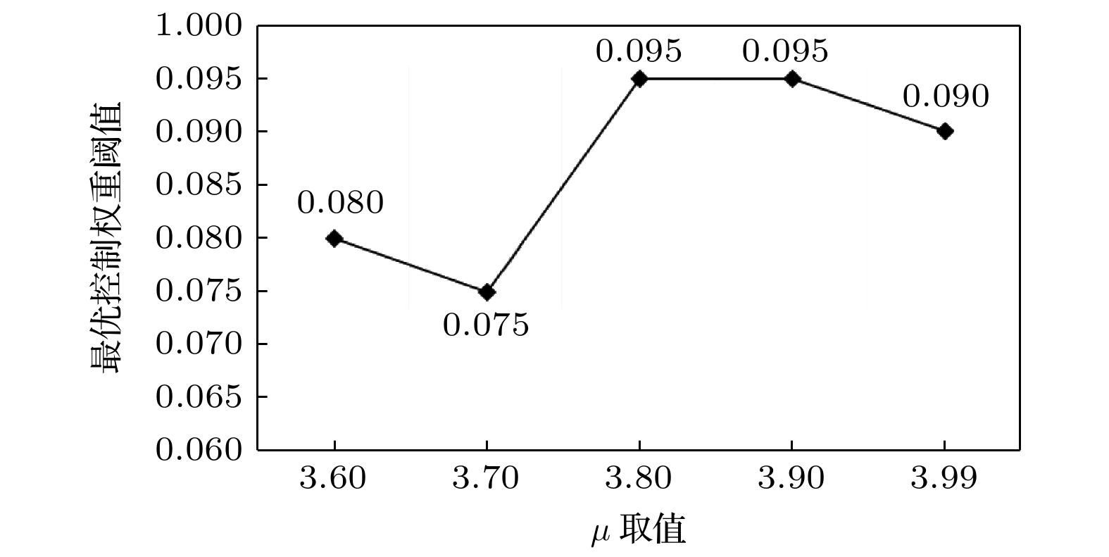
图 6 不同混沌状态对应的最优权重阈值变化
Fig. 6. The change of optimal weight threshold corresponding to different chaotic states.
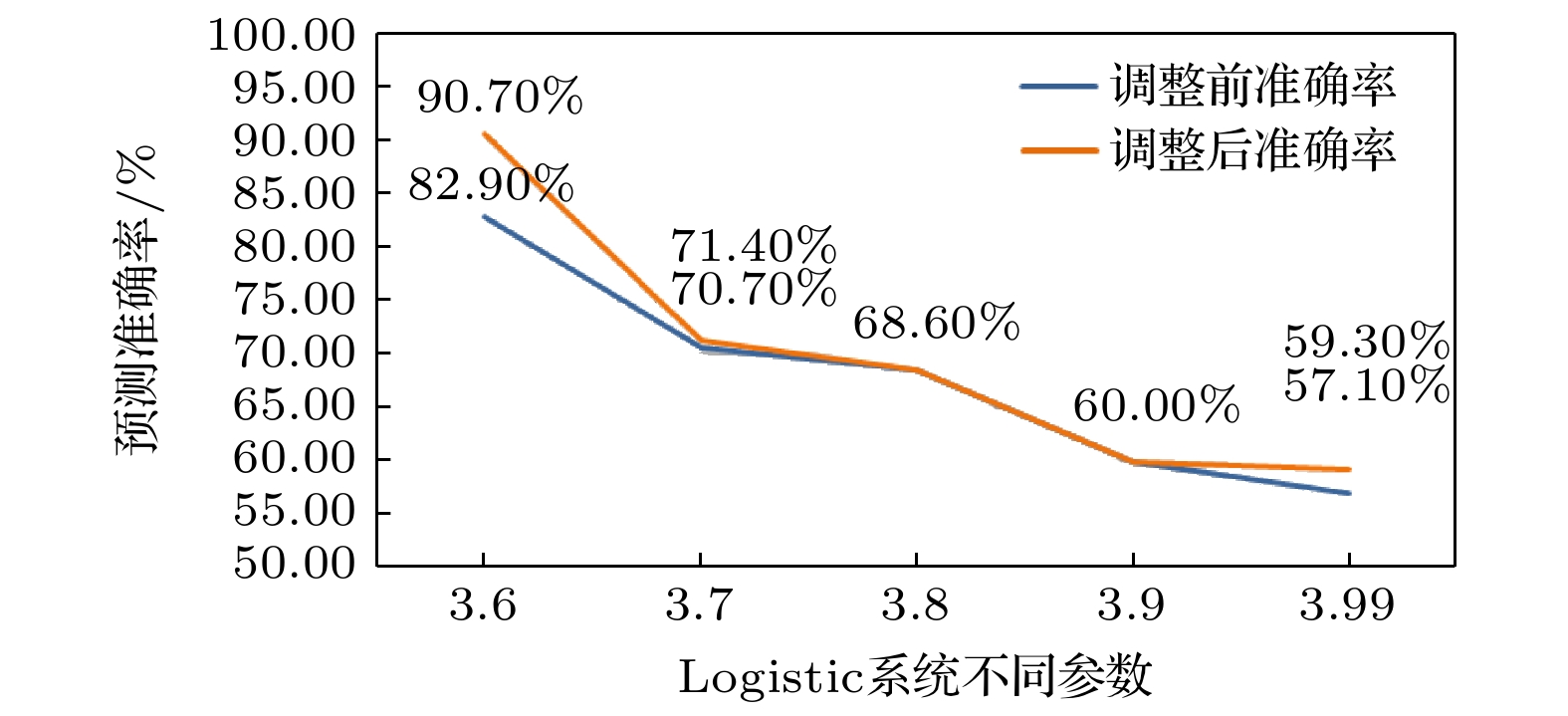
图 7 不同混沌状态对应的预测准确率变化
Fig. 7. The change of prediction accuracy of different chaotic states.
表 1 模型参数及结果
Table 1. Parameters and results of the models.
模型 train test win L1 L2 D1 D2 准确率 Logistic
(μ = 3.6)5000 15 22 16 4 4 1 82.90% Logistic
(μ = 3.7)5000 15 22 16 4 4 1 70.70% Logistic
(μ = 3.8)5000 15 2 20 4 4 1 68.60% Logistic
(μ = 3.9)5000 15 2 16 4 2 1 60.00% Logistic
(μ = 3.99)5000 15 2 16 4 4 1 57.10% Henon 5000 15 2 22 2 2 1 67.10% Rossler 5000 15 2 16 4 4 1 77.10%  下载: 导出CSV
表 2 权重结构拆分
Table 2. Weight structure resolution.
结构 起始点 终点 input_gate 0 units forget_gate units 2×units cell 2×units 3×units output_gate 3×units 4×units
下载: 导出CSV
表 3 输出门权重矩阵图
Table 3. Heat diagram of output door’s weights.
w1 w2 w3 w4 w5 w6 w7 w8 w9 w10 w11 w12 w13 w14 w15 w16 x1 0.032129 0.144328 0.007293 0.003557 0.070465 0.011652 0.11142 0.048287 0.105727 0.039649 0.010162 0.119949 0.0771 0.126937 0.001947 0.089396 x2 0.070867 0.013232 0.054503 0.073496 0.005734 0.064071 0.145835 0.083217 0.025553 0.033065 0.113584 0.028327 0.054085 0.177761 0.010123 0.046546 x3 0.083647 0.046366 0.066226 0.044534 0.010054 0.077919 0.071001 0.018548 0.035294 0.071642 0.053888 0.028448 0.102273 0.096744 0.078535 0.114879 x4 0.039123 0.113002 0.161581 0.113866 0.070651 0.085571 0.01836 0.015408 0.032978 0.018375 0.068342 0.059137 0.00701 0.070451 0.032602 0.099853 x5 0.013762 0.055823 0.147481 0.055493 0.093444 0.027264 0.082384 0.058674 0.032903 0.033342 0.045937 0.035937 0.110378 0.004487 0.161653 0.041037 x6 0.038079 0.089649 0.013102 0.021696 0.042833 0.109787 0.001024 0.0673 0.036916 0.134038 0.066291 0.146953 0.009803 0.081372 0.098701 0.042456 x7 0.013865 0.001702 0.057869 0.072264 0.104456 0.029761 0.062669 0.07539 0.05715 0.102282 0.017876 0.012626 0.020022 0.100243 0.153076 0.11875 x8 0.002042 0.006925 0.060008 0.13031 0.136406 0.056203 0.061606 0.028064 0.006926 0.099129 0.055122 0.117276 0.06846 0.014505 0.078184 0.078834 x9 0.044205 0.171724 0.153162 0.13818 0.029189 0.025947 0.049391 0.012338 0.100584 0.028133 0.004946 0.017914 0.008463 0.014741 0.066944 0.134139 x10 0.094619 0.0563 0.040223 0.096283 0.10152 0.145036 0.051991 0.075623 0.075216 0.061209 0.057986 0.066076 0.004787 0.01945 0.042341 0.011339 x11 0.078909 0.005603 0.08149 0.125202 0.069081 0.10143 0.122451 0.027058 0.057647 0.016226 0.03275 0.050667 0.036795 0.11072 0.081767 0.002204 x12 0.046159 0.005688 0.006237 0.004618 0.014815 0.005272 0.04598 0.037005 0.190933 0.065535 0.005131 0.015155 0.065812 0.099804 0.172294 0.21956 x13 0.111226 0.027026 0.027497 0.074868 0.139154 0.084413 0.080342 0.038769 0.088824 0.047083 0.056548 0.002081 0.10549 0.049929 0.020529 0.04622 x14 0.092772 0.03999 0.055938 0.128114 0.036386 0.013061 0.083943 0.051033 0.106374 0.007257 0.063049 0.091929 0.084821 0.020458 0.089496 0.035379 x15 0.131586 0.038161 0.176303 0.041758 0.049173 0.096633 0.0033 0.045529 0.084262 0.050839 0.003322 0.063406 0.029601 0.045323 0.116047 0.024757 x16 0.070289 0.05378 0.092472 0.03372 0.052087 0.110236 0.055639 0.124221 0.029371 0.06142 0.04904 0.043376 0.012261 0.041226 0.109564 0.061299 均
值0.060205 0.054331 0.075087 0.072372 0.064091 0.065266 0.065459 0.050404 0.066666 0.054326 0.043998 0.056204 0.049428 0.067134 0.082113 0.072915
下载: 导出CSV
表 4 μ = 3.99时不同参数的预测准确率
Table 4. The prediction accuracy of different parameters when μ = 3.99.
指标 调整前 以各权重阀值调整后 变化趋势 0.09 0.1 0.11 L1 16 15 12 10 
准确率 57.10% 59.30% 56.40% 51.40%  下载: 导出CSV
表 5 神经元数及预测准确率变化表
Table 5. Table of neuron numbers and prediction accuracy.
模型 调整前L1 调整后L1 调整前准确率 调整后准确率 神经元数调整 准确率变化趋势 Logistic
(μ = 3.6)16 15 82.90% 90.70% –1 
Logistic
(μ = 3.7)16 13 70.70% 71.40% –3 
Logistic
(μ = 3.8)20 16 68.60% 68.60% –4 
Logistic
(μ = 3.9)16 12 60.00% 60.00% –4 
Logistic
(μ = 3.99)16 15 57.10% 59.30% –1 
Henon 22 21 67.10% 70.00% –1 
Rossler 16 14 77.10% 83.60% –2  下载: 导出CSV
表 6 μ = 3.6 时不同参数的预测准确率
Table 6. The prediction accuracy of different parameters when μ = 3.6.
指标 调整前 以各权重阀值调整后 变化趋势 0.08 0.09 0.095 L1 16 15 12 10 
准确率 82.90% 90.70% 87.90% 78.60%  下载: 导出CSV
表 7 μ = 3.7 时不同参数的预测准确率
Table 7. The prediction accuracy of different parameters when μ = 3.7.
指标 调整前 以各权重阀值调整后 变化趋势 0.075 0.09 0.105 L1 16 13 11 9 
准确率 70.70% 71.40% 65.00% 60.70%  下载: 导出CSV
表 8 μ = 3.8时不同参数的预测准确率
Table 8. The prediction accuracy of different parameters when μ = 3.8.
指标 调整前 以各权重阀值调整后 变化趋势 0.085 0.095 0.105 L1 20 18 16 12 
准确率 68.60% 68.60% 68.60% 65.00%  下载: 导出CSV
表 9 μ = 3.9 时不同参数的预测准确率
Table 9. The prediction accuracy of different parameters when μ = 3.9.
指标 调整前 以各权重阀值调整后 变化趋势 0.09 0.095 0.1 L1 16 14 12 10 
准确率 60.00% 60.00% 60.00% 55.00%  下载: 导出CSV
表 10 Henon系统取不同参数的预测准确率
Table 10. Prediction accuracy of Henon system for different parameters.
指标 调整前 以各权重阀值调整后 变化趋势 0.1 0.11 0.12 0.14 L1 22 21 19 16 14 
准确率 67.10% 70.00% 66.40% 65.70% 65.00%  下载: 导出CSV
表 11 Rossler系统取不同参数的预测准确率
Table 11. Prediction accuracy of Rossler system for different parameters.
指标 调整前 以各权重阀值调整后 变化趋势 0.085 0.095 0.105 0.115 L1 16 14 12 11 8 
准确率 77.10% 83.60% 81.40% 80.70% 71.40%  下载: 导出CSV
-
[1] 邓帅 2019 计算机应用研究 36 1984
Deng S 2019 Appl. Res. Comput. 36 1984
[2] 邵恩泽, 吴正勇, 王灿 2020 工业控制计算机 33 11
Google Scholar
Shao E Z, Wu Z Y, Wang C 2020 Ind. Contrl. Comput. 33 11
Google Scholar
[3] 乔俊飞, 樊瑞元, 韩红桂, 阮晓钢 2010 控制理论与应用 27 111
Qiao J F, Fan R Y, Han H G, Ruan X G 2010 Contl. Theor. Appl. 27 111
[4] 陈国茗, 于腾腾, 刘新为 2021 数值计算与计算机应用 42 215
Google Scholar
Chen G M, Yu T T, Liu X W 2021 J. Num. Method. Comp. Appl. 42 215
Google Scholar
[5] 魏德志, 陈福集, 郑小雪 2015 物理学报 64 110503
Google Scholar
Wei D Z, Chen F J, Zheng X X 2015 Acta Phys. Sin. 64 110503
Google Scholar
[6] 王新迎, 韩敏 2015 物理学报 64 070504
Google Scholar
Wang X Y, Han M 2015 Acta Phys. Sin 64 070504
Google Scholar
[7] 黄伟建, 李永涛, 黄远 2021 物理学报 70 010501
Google Scholar
Huang W J, Li Y T, Huang Y 2021 Acta Phys. Sin. 70 010501
Google Scholar
[8] Yamaguti Y, Tsuda I 2021 Chaos 31 013137
Google Scholar
[9] Graves A 2013 arXiv: 1308.0850 [cs. NE]
[10] Johnston D E 1978 Proc 8 th BHRA Int Conf Fluid Sealing Durham, UK, 1978 pC1-1
[11] Sezer O B, Gudelek M U, Ozbayoglu A M 2020 Appl. Soft Comput. J. 90 106181
Google Scholar
[12] 甘文娟, 陈永红, 韩静, 王亚飞 2020 计算机系统应用 29 212
Google Scholar
Gan W J, Chen Y H, Han J, Wang Y F 2020 Comput. Syst. Appl. 29 212
Google Scholar
[13] Farmelo G 2002 It Must Be Beautiful: Great Equations of Modern Science (London: Granta Publications) pp28–45
[14] Grassberger P, Procaccia I 1983 Physica D 9 189
Google Scholar
[15] Nauenberg M 1983 Ann. N. Y. Acad. Sci. 410 317
Google Scholar
[16] 张中华, 丁华福 2009 计算机技术与发展 19 185
Google Scholar
Zhang Z H, Ding H F 2009 Comput. Technol. Dev. 19 185
Google Scholar
[17] Butcher J C 1967 J. ACM 14 84
Google Scholar
[18] Liu C, Yin S Q, Zhang M, Zeng Y, Liu J Y 2014 Appl. Mech. Mater. 644-650 2216
[19] Bao Y K, Liu Z T 2006 LNCS 4224 504
[20] Ou Y Y, Chen G H, Oyang Y J 2006 LNCS 4099 1017

 下载:
下载:


计量
- 文章访问数: 7680
- PDF下载量: 88
- 被引次数: 0
