


-
Fractal lattices are a special kind of lattice: they have non-integer Hausdorff dimensions and break the translation invariance. Studying these lattices can help us understand the influence of non-integer dimensions and lacking of translational symmetry on critical behaviors. We study the Ising model in a fractal lattice with a non-integer dimension of
$\log_4(12)\approx 1.7925$ by using the higher order tensor network renormalization group (HOTRG) algorithm. The partition function is represented in terms by a tensor network, and is finally calculated by a coarse graining process based on higher order singular value decomposition. When the truncation length and the time of coarse graining increase, the results are found convergent. Magnetic moment, internal energy and correlation properties are calculated by inserting impurity tensors into the tensor network at different temperatures and in different external magnetic fields. The magnetic susceptibility is obtained by differentiating the magnetic moment with respect to the magnetic field, and the capacity is calculated by differentiating the internal energy with respect to the temperature. Our numerical results show that there is a continuous order-disorder phase transition in this system, and the critical temperature is found to be$T_{\rm{c}}/J = 1.317188$ . Physical quantities show singular behaviours around the critical point, and the correlation length is found to be divergent at the critical point, which is consistent with the result of the renormalization group theory. The corresponding critical exponent is obtained by fitting the numerical data around the critical point. We also calculate the critical exponents at different positions by inserting impurity tensors into different places of the lattice. Owing to the lack of translational symmetry, it is found that the critical exponents α, β, δ fitted at different positions vary, but the critical exponent γ remains almost the same. From the scaling hypothesis, it can be deduced that the critical exponents satisfy the hyperscaling relations which contain the dimension of the lattice. Our numerical results show that all of the hyperscaling relations are satisfied when the fractional dimension and the critical exponents we have obtained are substituted into them on some sites of the fractal lattice, but only two of the four hyperscaling relations are satisfied on other sites.-
Keywords:
- fractal lattice /
- Ising model /
- tensor network /
- critical phenomena
[1] Fisher M E 1974 Rev. Mod. Phys. 46 597
 Google Scholar
[2] Kadanoff L P 1985 Physics 2 263
[3] Efrati E, Wang Z, Kolan A, Kadanoff L P 2014 Rev. Mod. Phys. 86 647
Google Scholar
[4] Kardar M 2007 Statistical Physics of Fields (Cambridge: Cambridge University Press) pp54–92
[5] Onsager L 1944 Phys. Rev. 65 117
Google Scholar
[6] Yang C N 1952 Phys. Rev. 85 808
Google Scholar
[7] Wilson K G, Kogut J 1974 Phys. Rep. 12 75
Google Scholar
[8] Gefen Y, Mandelbrot B B, Aharony A 1980 Phys. Rev. Lett. 45 855
Google Scholar
[9] Gefen Y, Meir Y, Mandelbrot B B, Aharony A 1983 Phys. Rev. Lett. 50 145
Google Scholar
[10] Gefen Y, Aharony A, Mandelbrot B B 1983 J. Phys. A: Math. Gen. 16 1267
Google Scholar
[11] Gefen Y, Aharony A, Mandelbrot B B 1984 J. Phys. A: Math. Gen. 17 1277
Google Scholar
[12] Gefen Y, Aharony A, Shapir Y, Mandelbrot B B 1984 J. Phys. A 17 435
Google Scholar
[13] Luscombe J H, Desai R C 1985 Phys. Rev. B 32 1614
[14] Stosic T, Stosic B D, Milosevic S, Stanley H E 1996 Physica A 233 31
Google Scholar
[15] Vezzani A 2003 J. Phys. A 36 1593
Google Scholar
[16] Carmona J M, Marini U, Marconi B, Ruiz-Lorenzo J J, Tarancon A 1998 Phys. Rev. B 58 14387
Google Scholar
[17] Levin M, Nave C P 2007 Phys. Rev. Lett. 99 120601
Google Scholar
[18] Gu Z C, Wen X G 2009 Phys. Rev. B 80 155131
Google Scholar
[19] Xie Z Y, Chen J, Qin M P, Zhu J W, Yang L P, Xiang T 2012 Phys. Rev. B 86 045139
Google Scholar
[20] Ueda H, Okunishi K, Nishino T 2014 Phys. Rev. B 89 075116
Google Scholar
[21] Evenbly G, Vidal G 2015 Phys. Rev. Lett. 115 180405
Google Scholar
[22] Evenbly G, Vidal G 2015 Phys. Rev. Lett. 115 200401
Google Scholar
[23] Evenbly G, Vidal G 2016 Phys. Rev. Lett. 116 040401
Google Scholar
[24] Hauru M, Evenbly G, Ho W W, Gaiotto D, Vidal G 2016 Phys. Rev. B 94 115125
Google Scholar
[25] Evenbly G 2017 Phys. Rev. B 95 045117
Google Scholar
[26] Yang S, Gu Z C, Wen X G 2017 Phys. Rev. Lett. 118 110504
Google Scholar
[27] Evenbly G 2018 Phys. Rev. B 98 085155
Google Scholar
[28] Adachi D, Okubo T, Todo S 2020 Phys. Rev. B 102 054432
Google Scholar
[29] Adachi D, Okubo T, Todo S 2022 Phys. Rev. B 105 L060402
Google Scholar
[30] Genzor J, Gendiar A, Nishino T 2016 Phys. Rev. E 93 012141
Google Scholar
[31] Genzor J, Gendiar A, Kao Y J 2022 Phys. Rev. E 105 024124
Google Scholar
[32] Krcmar R, Genzor J, Lee Y, Cencarikova H, Nishino T, Gendiar A 2018 Phys. Rev. E 98 062114
[33] Yang Z, Lustig E, Lumer Y, Segev M 2020 Light Sci. Appl. 9 128
Google Scholar
[34] Manna S, Nandy S, Roy B 2022 Phys. Rev. B 105 201301
Google Scholar
[35] Pai S, Prem A 2019 Phys. Rev. B 100 155135
Google Scholar
[36] Ann H, Dennis G 1971 Statistics: A Foundation for Analysis (Addison-Wesley) pp344–348
-
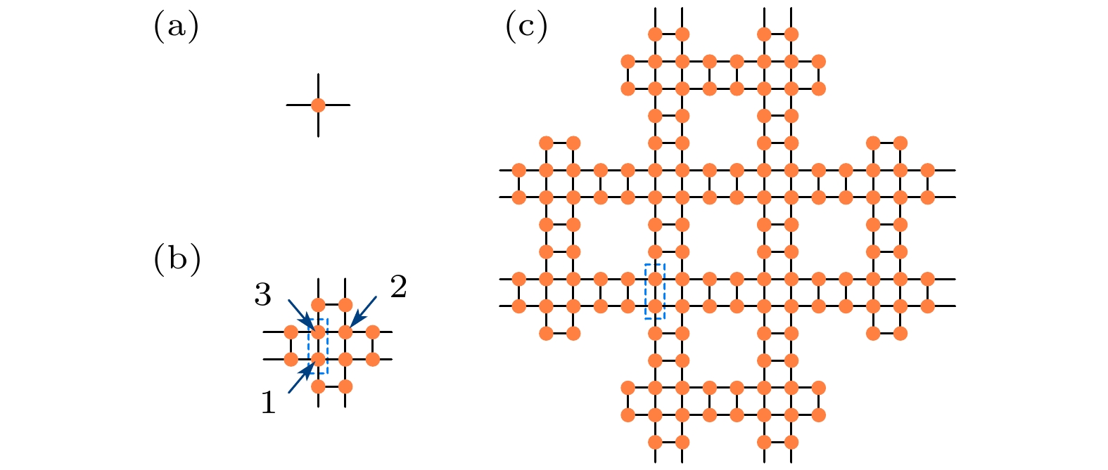
图 1 分形格点 (a) 单个自旋; (b) 12个自旋连接在一起组成团簇; (c) 图(b)的团簇替换图(b)中的格点得到的新的团簇. 其中橙色的点表示自旋, 他们之间的连线表示自旋之间的伊辛相互作用
Fig. 1. Fractal lattice: (a) A single spin; (b) 12 spins are joined together to form a cluster; (c) each site in the cluster shown in panel (b) is replaced with the entire cluster in panel (b), yielding the new cluster. The orange dots indicate spins and the lines between them indicate the Ising interaction between them

图 3 粗粒化过程的图形表示, 从张量
$ {\boldsymbol{U}}_x $ ,$ {\boldsymbol{U}}_y $ ,$ {\boldsymbol{T}}^{(n)} $ ,$ {\boldsymbol{X}}^{(n)} $ $ {\boldsymbol{Y}}^{(n)} $ ,$ {\boldsymbol{C}}^{(n)} $ 出发, 对张量网络求和缩并得到(a)$ {\boldsymbol{T}}^{(n+1)} $ , (b)$ {\boldsymbol{Y}}^{(n+1)} $ , (c)$ {\boldsymbol{X}}^{(n+1)} $ , (d)$ {\boldsymbol{C}}^{(n+1)} $ Fig. 3. Graphical representations of the coarse graining processes. Obtaining the tensors (a)
${\boldsymbol{ T}}^{(n+1)} $ , (b)$ {\boldsymbol{Y}}^{(n+1)} $ , (c)$ {\boldsymbol{X}}^{(n+1)} $ and (d)$ {\boldsymbol{C}}^{(n+1)} $ by contracting the tensor networks consisting of$ {\boldsymbol{U}}_x $ ,$ {\boldsymbol{U}}_y $ ,$ {\boldsymbol{T}}^{(n)} $ ,$ {\boldsymbol{X}}^{(n)} $ ,$ {\boldsymbol{Y}}^{(n)} $ and$ {\boldsymbol{C}}^{(n)} $ 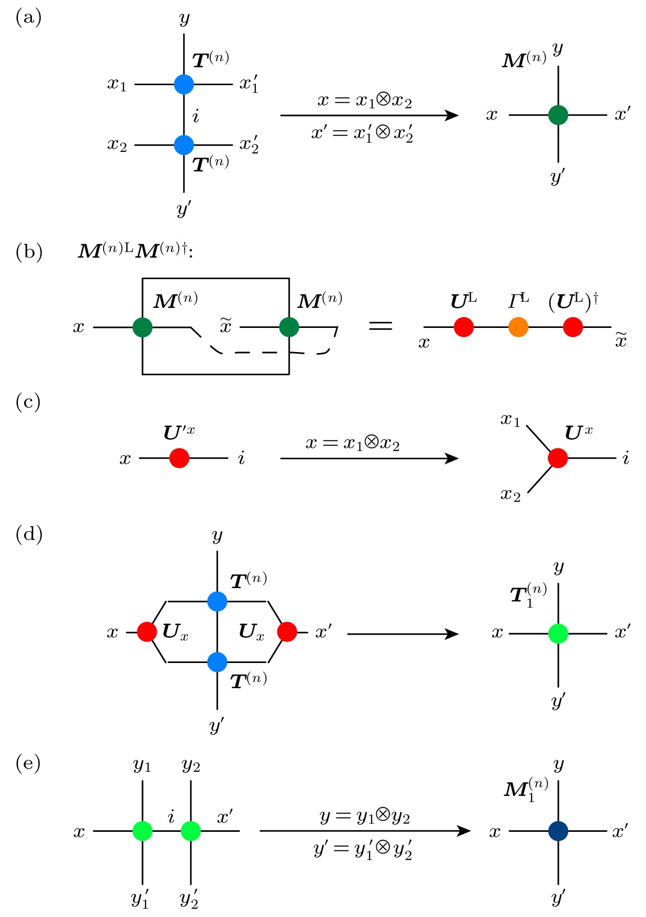
图 2 HOTRG张量重正化群计算过程的图形表示 (a)将两个
$ {\boldsymbol{T}}^{(n)} $ 张量的上下指标求和得到张量$ {\boldsymbol{M}}^{(n)} $ , 在这里有$ x=x_1\otimes x_2 $ ,$ x' =x_1' \otimes x_2' $ ,$ x_1 $ ,$ x_2 $ 合为了指标x,$ x_1' $ ,$ x_2' $ 合为了指标$ x' $ ; (b)对$ {\boldsymbol{M}}^{(n){\rm{L}}}\left( {\boldsymbol{M}}^{(n){\rm{L}}}\right)^{\dagger} $ 奇异值分解得到$ {\boldsymbol{U}}^{\rm{L}} $ ,$ {\boldsymbol{\varGamma}}^{\rm{L}} $ ; (c)将$ {\boldsymbol{U}}^{\rm{L}} $ 的x指标拆分成$ x_1 $ ,$ x_2 $ 指标得到$ {\boldsymbol{U}}'^{\rm{L}} $ ; (d)将两个$ {\boldsymbol{T}}^{(n)} $ 张量, 两个$ {\boldsymbol{U}}^x $ 张量求和缩并得到张量$ {\boldsymbol{T}}^{(n)}_1 $ ; (e)将两个${\boldsymbol{ T}}^{(n)}_1 $ 张量左右相连得到$ {\boldsymbol{M}}^{(n)}_1 $ , 在这里有$y=y_1\otimes $ $ y_2$ ,$ y' =y_1'\otimes y_2' $ ,$ y_1 $ ,$ y_2 $ 合为了指标y,$ y_1' $ ,$ y_2' $ 合为了指标$ y' $ Fig. 2. Graphical representations of HOTRG renormalization steps: (a) Determination of tensor
$ {\boldsymbol{M}}^{(n)} $ by contracting two$ {\boldsymbol{T}}^{(n)} $ tensors. Here, indexes$ x_1 $ ,$ x_2 $ are combined into index x and$ x_1' $ ,$ x_2' $ are combined into$ x' $ ($ x=x_1\otimes x_2 $ ,$ x' =x_1' \otimes x_2' $ ,$ x_1 $ ,$ x_2 $ ); (b) performing a singular value decomposition of matrix$ {\boldsymbol{M}}^{(n){\rm{L}}}\left( {\boldsymbol{M}}^{(n){\rm{L}}}\right)^{\dagger} $ to obtain matrices$ {\boldsymbol{U}}^{\rm{L}} $ and$ {\boldsymbol{\varGamma}}^{\rm{L}} $ ; (c) dividing the index x of$ {\boldsymbol{U}}'^x $ into$ x_1 $ and$ x_2 $ to obtain tensor$ {\boldsymbol{U}}^x $ ; (d) determination of tensor$ {\boldsymbol{T}}^{(n)}_1 $ by contracting two$ {\boldsymbol{T}}^{(n)} $ and two$ {\boldsymbol{U}}^x $ tensors; (e) determination of tensor$ {\boldsymbol{M}}^{(n)} $ by contracting two$ {\boldsymbol{T}}^{(n)} $ tensors. Here, indexes$ x_1 $ ,$ x_2 $ are combined into index x and$ x_1' $ ,$ x_2' $ are combined into$ x' $ ($ x=x_1\otimes x_2 $ ,$ x' =x_1' \otimes x_2' $ ,$ x_1 $ ,$ x_2 $ )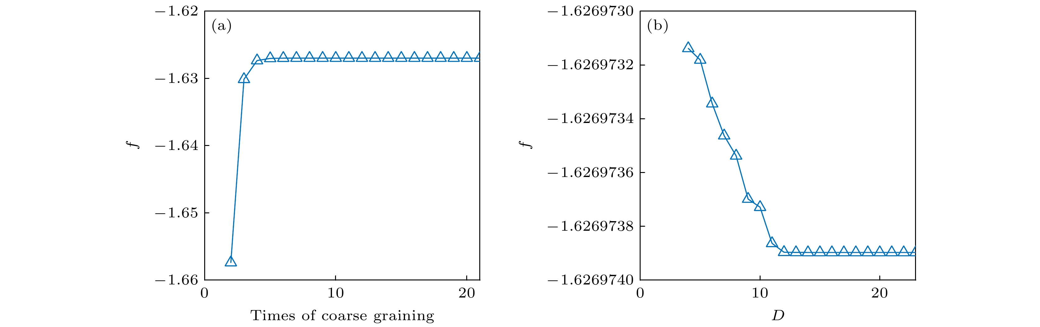
图 4 在临界温度处, 系统平均自由能随(a)粗粒化次数(截断长度D = 24)以及(b)随截断长度D(粗粒化次数为20)的变化关系图
Fig. 4. Average free energy calculated by HOTRG method at the critical point (a) as a function of coarse graining times (truncation lengths are chosen as
$ D = 24 $ ) and (b) as a function of truncation lengths D (coarse graining times are chosen as 20)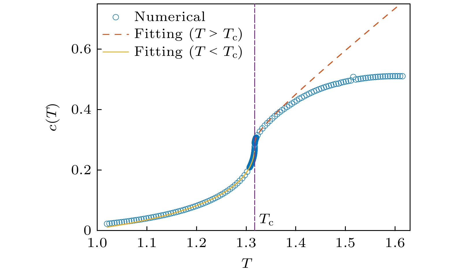
图 5 比热随温度变化的关系图. 其中蓝色的圈表示利用HOTRG数值计算得到的结果, 计算选取的截断长度为D = 16. 黄色的实线和红色的虚线分别表示
$T < T_{\rm{c}}$ 和$T > T_{\rm{c}}$ 时对(24)式的拟合结果, 紫色虚线标出的是临界温度所在位置, 其大小为$T_{\rm{c}} = 1.317188$ Fig. 5. Capacity as a function of temperature. The numerical results calculated by HOTRG methods are depicted as blue circles (the truncation length is chosen as
$ D = 16 $ ). The yellow solid line (red dashed line) is a fitting curve for Eq.(24) when$T < T_{\rm{c}}$ ($T > T_{\rm{c}}$ ). The vertical purple dashed line shows the location of the critical temperature$T_{\rm{c}} = $ $ 1.317188$ 
图 6 不同截断长度D下利用HOTRG算法确定出的临界温度
$T_{\rm{c}}$ Fig. 6. The critical temperatures determined by HOTRG method as a function of the truncation lengths D

图 7 比热的奇异部分
$c_{\rm{c}}$ 随约化温度t变化的关系图. 其中蓝色星号表示利用HOTRG求得的数值结果, 红色的虚线表示对(24)式拟合的结果, 横轴和纵轴采用的都是对数坐标Fig. 7. Singular part of the capacity
$c_{\rm{c }}$ as a function of reduced temperature t. Numerical results obtained by HOTRG method are depicted by blue stars, and the red dashed line is a fitting curve for Eq.(24). Both the horizontal coordinate and the vertical coordinate are logarithmic here
图 8 不同约化温度区间
$ [t_{{\rm{ub}}}/120, t_{{\rm{ub}}}] $ 下临界指数α((24)式)的拟合结果及误差. 其中蓝色的线表示α的拟合结果, 红色的线表示拟合的误差$ 1-R^2 $ . 横轴和右边的纵轴$ 1-R^2 $ 采用的是对数坐标. 误差棒表示拟合参数置信度为95%的置信区间Fig. 8. The fitting results (blue) and errors
$ 1-R^2 $ (red) for the critical exponent α (Eq. (24)) at different induced temperature intervals$ [t_{{\rm{ub}}}/120, t_{{\rm{ub}}}] $ . The horizontal coordinate and the right vertical coordinate$ 1-R^2 $ are logarithmic here. The error bars represent the confidence intervals with a confidence level of 95% for the fitted parameter
图 9 在临界温度下, 磁矩随外加磁场h变化的关系图. 其中蓝色的点表示利用HOTRG计算得到的结果, 红色的实线表示对(27)式的拟合结果. 其中横轴与纵轴采用的都是对数坐标
Fig. 9. Magnetic moment as a function of the external magnetic field h at the critical temperature. The blue dots show the numerical results obtained by HOTRG method, and the red solid line is a fitting curve for Eq. (27). Both the horizontal coordinate and the vertical coordinate are logarithmic here
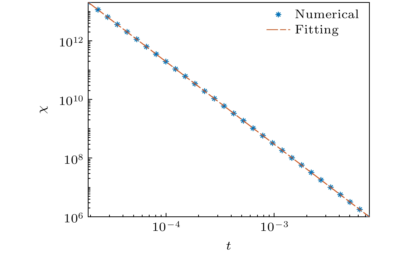
图 10 在
$ T > T_{\rm{c}} $ 时, 磁化率随约化温度t变化的关系图. 其中蓝色的星号表示利用HOTRG计算得到的结果, 红色的虚线表示利用(29)式进行拟合的结果. 其中横轴与纵轴采用的都是对数坐标Fig. 10. Magnetic susceptibility as a function of the reduced temperature t when
$ T > T_{\rm{c }}$ . The blue stars show the numerical results obtained by HOTRG method, and the red dashed line is a fitting curve for Eq. (29). Both the horizontal coordinate and the vertical coordinate are logarithmic here
图 11 在
$ T < T_{\rm{c}} $ 时, 自发磁矩随约化温度t变化的关系图. 其中蓝色的星号表示利用HOTRG计算得到的结果, 红色的虚线表示对(30)式进行拟合的结果. 其中横轴与纵轴采用的都是对数坐标Fig. 11. Spontaneous magnetic moment as a function of the reduced temperature t when
$ T < T_{\rm{c }}$ . The blue stars show the numerical results obtained by the HOTRG method and the red dashed line is a fitting curve for Eq.(30). Both the horizontal coordinate and the vertical coordinate are logarithmic
图 12 在
$T > T_{\rm{c}}$ 时, 自旋-自旋关联函数随距离变化的关系图. 其中不同颜色的点表示不同温度下HOTRG的计算结果, 不同颜色的实线表示不同温度下对(31)式进行拟合的结果, 不同颜色的虚线标出了不同温度下拟合得到的关联长度. 其中横轴采用的是对数坐标Fig. 12. The spin-spin correlation funcitons as a function of the distance r when
$ T > T_{\rm{c}} $ . The dots show the numerical results obtained by HOTRG method. The solid lines are fitting curves for Eq.(31). The vertical dashed lines show the locations of the correlation lengths. Different colors mean different deduced temperatures. The horizontal coordinate is logarithmic here
图 13 在
$ T > T_{\rm{c}} $ 时, 不同约化温度t下关联长度ξ与指数$ d+\eta-2 $ 的拟合结果. 其中蓝色的圈表示$ d+\eta-2 $ 的拟合结果, 红色的星号表示ξ的拟合结果, 红色的虚线表示对(32)式进行拟合的结果. 其中横轴t和纵轴ξ采用了对数坐标. 误差棒表示拟合参数置信度为95%的置信区间Fig. 13. Fitting results for correlation lengths ξ (blue circles) and the exponent
$ d+\eta-2 $ (red stars) at different reduced temperatures t. The red dashed line is a fitting curve for Eq.(32). The horizontal coordinate t and the right vertical coordinate ξ are logarithmic here. The error bars represent the confidence intervals with a confidence level of 95% for the fitted parameter
图 14 在位置
$ P(n) $ 处拟合得到的临界指数(a) α, (b) β, (c) δ和(d) γ随n的变化关系图. 误差棒表示拟合参数置信度为95%的置信区间Fig. 14. Ffitting results for the critical exponents (a) α, (b) β, (c) δ and (d) γ at different positions
$ P(n) $ as functions of n. The error bars represent the confidence intervals with a confidence level of 95% for the fitted parameter表 1 在
$P(1)$ 位置拟合得到的的临界指数.Table 1. Critical exponents fitted at position
$P(1)$ 临界指数 α β γ δ η ν 拟合结果 –0.8290 0.0138 2.816 205.0 0.2325 1.5986  下载: 导出CSV
-
[1] Fisher M E 1974 Rev. Mod. Phys. 46 597
Google Scholar
[2] Kadanoff L P 1985 Physics 2 263
[3] Efrati E, Wang Z, Kolan A, Kadanoff L P 2014 Rev. Mod. Phys. 86 647
Google Scholar
[4] Kardar M 2007 Statistical Physics of Fields (Cambridge: Cambridge University Press) pp54–92
[5] Onsager L 1944 Phys. Rev. 65 117
Google Scholar
[6] Yang C N 1952 Phys. Rev. 85 808
Google Scholar
[7] Wilson K G, Kogut J 1974 Phys. Rep. 12 75
Google Scholar
[8] Gefen Y, Mandelbrot B B, Aharony A 1980 Phys. Rev. Lett. 45 855
Google Scholar
[9] Gefen Y, Meir Y, Mandelbrot B B, Aharony A 1983 Phys. Rev. Lett. 50 145
Google Scholar
[10] Gefen Y, Aharony A, Mandelbrot B B 1983 J. Phys. A: Math. Gen. 16 1267
Google Scholar
[11] Gefen Y, Aharony A, Mandelbrot B B 1984 J. Phys. A: Math. Gen. 17 1277
Google Scholar
[12] Gefen Y, Aharony A, Shapir Y, Mandelbrot B B 1984 J. Phys. A 17 435
Google Scholar
[13] Luscombe J H, Desai R C 1985 Phys. Rev. B 32 1614
[14] Stosic T, Stosic B D, Milosevic S, Stanley H E 1996 Physica A 233 31
Google Scholar
[15] Vezzani A 2003 J. Phys. A 36 1593
Google Scholar
[16] Carmona J M, Marini U, Marconi B, Ruiz-Lorenzo J J, Tarancon A 1998 Phys. Rev. B 58 14387
Google Scholar
[17] Levin M, Nave C P 2007 Phys. Rev. Lett. 99 120601
Google Scholar
[18] Gu Z C, Wen X G 2009 Phys. Rev. B 80 155131
Google Scholar
[19] Xie Z Y, Chen J, Qin M P, Zhu J W, Yang L P, Xiang T 2012 Phys. Rev. B 86 045139
Google Scholar
[20] Ueda H, Okunishi K, Nishino T 2014 Phys. Rev. B 89 075116
Google Scholar
[21] Evenbly G, Vidal G 2015 Phys. Rev. Lett. 115 180405
Google Scholar
[22] Evenbly G, Vidal G 2015 Phys. Rev. Lett. 115 200401
Google Scholar
[23] Evenbly G, Vidal G 2016 Phys. Rev. Lett. 116 040401
Google Scholar
[24] Hauru M, Evenbly G, Ho W W, Gaiotto D, Vidal G 2016 Phys. Rev. B 94 115125
Google Scholar
[25] Evenbly G 2017 Phys. Rev. B 95 045117
Google Scholar
[26] Yang S, Gu Z C, Wen X G 2017 Phys. Rev. Lett. 118 110504
Google Scholar
[27] Evenbly G 2018 Phys. Rev. B 98 085155
Google Scholar
[28] Adachi D, Okubo T, Todo S 2020 Phys. Rev. B 102 054432
Google Scholar
[29] Adachi D, Okubo T, Todo S 2022 Phys. Rev. B 105 L060402
Google Scholar
[30] Genzor J, Gendiar A, Nishino T 2016 Phys. Rev. E 93 012141
Google Scholar
[31] Genzor J, Gendiar A, Kao Y J 2022 Phys. Rev. E 105 024124
Google Scholar
[32] Krcmar R, Genzor J, Lee Y, Cencarikova H, Nishino T, Gendiar A 2018 Phys. Rev. E 98 062114
[33] Yang Z, Lustig E, Lumer Y, Segev M 2020 Light Sci. Appl. 9 128
Google Scholar
[34] Manna S, Nandy S, Roy B 2022 Phys. Rev. B 105 201301
Google Scholar
[35] Pai S, Prem A 2019 Phys. Rev. B 100 155135
Google Scholar
[36] Ann H, Dennis G 1971 Statistics: A Foundation for Analysis (Addison-Wesley) pp344–348


 下载:
下载:


计量
- 文章访问数: 8263
- PDF下载量: 218
- 被引次数: 0
