


-
位于动理学热离子带隙附近的低频阿尔芬扰动因可以与高能量粒子或背景热粒子发生相互作用而引起了广泛的关注. 本文在一般鱼骨模色散关系的理论框架下, 针对反磁剪切托卡马克等离子体中观测到的由高能量粒子或者背景热粒子激发的低频剪切阿尔芬波的线性特性进行了一系列的理论研究. 由于这些低频剪切阿尔芬波与2019年DIII-D开展的专门研究高能量离子驱动低频不稳定的实验密切相关, 因此本文通过采用DIII-D具有代表性实验的平衡参数, 证明了实验上观测的低频模和比压阿尔芬本征模分别是以阿尔芬极化为主的反应型和耗散型不稳定模, 因此, 将前者称为低频阿尔芬模更准确. 由于受逆磁和捕获粒子动理学效应的影响, 低频阿尔芬模既可以在低频区(频率小于热离子的渡越或反弹频率)与比压阿尔芬声模耦合, 又可以在高频区(频率大于或近似等于热离子的渡越频率)与比压阿尔芬本征模耦合. 此外, 由于受到不同激发机制的影响, 与局域在安全因子最小值有理面附近的低频阿尔芬模相比, 驱动比压阿尔芬本征模的高能量离子的压强梯度在偏离安全因子最小值的有理面时达到最大值, 相应的比压阿尔芬本征模的本征函数在高能量离子驱动最大的径向位置处出现峰值. 通过改变安全因子最小值理论上重现了实验上观测的比压阿尔芬本征模和低频阿尔芬模的上升频谱特征. 研究还表明, 比压阿尔芬声模由于受到强烈的朗道阻尼, 因而很难被高能量粒子激发, 这与基于第一性原理的理论预测和模拟结果一致. 本文证明了一般鱼骨模色散关系在解释和预测实验和数值模拟结果方面的强大能力.The low-frequency Alfvénic fluctuations in the kinetic thermal-ion gap frequency range have aroused the interest of researchers since they can interact with background thermal particles and/or energetic particles. In the theoretical framework of the general fishbone-like dispersion relation (GFLDR), we theoretically investigate and delineate the linear wave properties of the low-frequency shear Alfvén wave excited by energetic and/or thermal particles observed in tokamak experiments with reversed magnetic shear. These low-frequency shear Alfvén waves are closely related to the dedicated experiment on energetic ion-driven low-frequency instabilities conducted on DIII-D in 2019. Therefore, adopting the representative experimental equilibrium parameters of DIII-D, in this work we demonstrate that the experimentally observed low-frequency modes and beta-induced Alfvén eigenmodes (BAEs) are, respectively, the reactive-type unstable mode and dissipative-type unstable mode, each with dominant Alfvénic polarization, thus the former being more precisely called low-frequency Alfvén modes (LFAMs). More specifically, due to diamagnetic and trapped particle effects, the LFAM can be coupled with the beta-induced Alfvén-acoustic mode (BAAE) in the low-frequency range (frequency much less than the thermal-ion transit frequency and/or bounce frequency), or with the BAE in the high frequency range (frequency higher than or comparable to the thermal-ion transit frequency), resulting in reactive-type instabilities. Moreover, due to different instability mechanisms, the maximal drive of BAEs occurs in comparison with LFAMs, when the minimum of the safety factor (
$ q_{\rm min} $ ) deviates from a rational number. Meanwhile, the BAE eigenfunction peaks at the radial position of the maximum energetic particle pressure gradient, resulting in a large deviation from the$ q_{\rm min} $ surface. The ascending frequency spectrum patterns of the experimentally observed BAEs and LFAMs can be theoretically reproduced by varying$ q_{\rm min} $ , and they can also be well explained based on the GFLDR. In particular, it is confirmed that the stability of the BAAE is not affected by energetic ions, which is consistent with the first-principle-based theory predictions and simulation results. The present analysis illustrates the solid predictive capability of the GFLDR and its practical applications in enhancing the ability to explain experimental and numerical simulation results.-
Keywords:
- low frequency shear Alfvén waves /
- energetic particles /
- instabilities /
- gyrokinetic
[1] Chen L, Zonca F 2016 Rev. Mod. Phys. 88 015008
 Google Scholar
[2] Heidbrink W W, Strait E J, Chu M S, et al. 1993 Phys. Rev. Lett. 71 855
Google Scholar
[3] Turnbull A D, Strait E J, Heidbrink W W, et al. 1993 Phys. Fluids B 5 2546
Google Scholar
[4] Chen L, Zonca F 2007 Nucl. Fusion 47 S727
Google Scholar
[5] Zonca F, Chen L, Santoro R A 1996 Plasma Phys. Control. Fusion 38 2011
Google Scholar
[6] Zonca F, Chen L, Dong J Q, et al. 1999 Phys. Plasmas 6 1917
Google Scholar
[7] Zonca F, Biancalani A, Chavdarovski I, et al. 2010 J. Phys. Conf. Ser. 260 012022
Google Scholar
[8] Chavdarovski I, Zonca F 2009 Plasma Phys. Control. Fusion 51 115001
Google Scholar
[9] Lauber P, Brudgam M, Curran D, et al. 2009 Plasma Phys. Control. Fusion 51 124009
Google Scholar
[10] Zonca F, Chen L, Falessi M V, et al. 2021 J. Phys. Conf. Ser. 1785 012005
Google Scholar
[11] Cheng C 1982 Phys. Fluids 25 1020
Google Scholar
[12] Tang W, Connor J, Hastie R 1980 Nucl. Fusion 20 1439
Google Scholar
[13] Biglari H, Chen L 1991 Phys. Rev. Lett. 67 3681
Google Scholar
[14] Zonca F, Chen L, Botrugno A, et al. 2009 Nucl. Fusion 49 085009
Google Scholar
[15] Gorelenkov N, Berk H, Fredrickson E, et al. 2007 Phys. Lett. A 370 70
Google Scholar
[16] Gorelenkov N N, Zeeland M A V, Berk H L, et al. 2009 Phys. Plasmas 16 056107
Google Scholar
[17] Cheng C Z, Chen L, Chance M S 1985 Ann. Phys. 161 21
Google Scholar
[18] Kimura H, Kusama Y, Saigusa M, et al. 1998 Nucl. Fusion 38 1303
Google Scholar
[19] Sharapov S E, Testa D, Alper B, et al. 2001 Phys. Lett. A 289 127
Google Scholar
[20] Zonca F, Chen L 2014 Phys. Plasmas 21 072120
Google Scholar
[21] Zonca F, Chen L 2014 Phys. Plasmas 21 072121
Google Scholar
[22] Lu Z X, Zonca F, Cardinali A 2012 Phys. Plasmas 19 042104
Google Scholar
[23] Berk H L, Pfirsch D 1980 J. Math. Phys. 21 2054
Google Scholar
[24] Connor J, Hastie R, Taylor J 1979 Proc. R. Soc. London, Ser. A 365 1
Google Scholar
[25] Zonca F, Buratti P, Cardinali A, et al. 2007 Nucl. Fusion 47 1588
Google Scholar
[26] Chen W, Ding X T, Yang Q W, et al. 2010 Phys. Rev. Lett. 105 185004
Google Scholar
[27] Ma R, Qiu Z, Li Y, et al. 2021 Nucl. Fusion 61 036014
Google Scholar
[28] Chavdarovski I, Zonca F 2014 Phys. Plasmas 21 052506
Google Scholar
[29] Falessi M V, Carlevaro N, Fusco V, et al. 2019 Phys. Plasmas 26 082502
Google Scholar
[30] Falessi M V, Carlevaro N, Fusco V, et al. 2020 J. Plasma Phys. 86 845860501
Google Scholar
[31] Sharapov S, Alper B, Berk H, et al. 2013 Nucl. Fusion 53 104022
Google Scholar
[32] Gorelenkov N, Pinches S, Toi K 2014 Nucl. Fusion 54 125001
Google Scholar
[33] Heidbrink W, Zeeland M V, Austin M, et al. 2021 Nucl. Fusion 61 016029
Google Scholar
[34] Heidbrink W, Zeeland M V, Austin M, et al. 2021 Nucl. Fusion 61 066031
Google Scholar
[35] Heidbrink W, Choi G, Zeeland M V, et al. 2021 Nucl. Fusion 61 106021
Google Scholar
[36] Curran D, Lauber P, Carthy P J M, et al. 2012 Plasma Phys. Control. Fusion 54 055001
Google Scholar
[37] Lauber P 2013 Phys. Rep. 533 33
Google Scholar
[38] Fasoli A, Brunner S, Cooper W, et al. 2016 Nat. Phys. 12 411
Google Scholar
[39] Bierwage A, Lauber P 2017 Nucl. Fusion 57 116063
Google Scholar
[40] Choi G, Liu P, Wei X, et al. 2021 Nucl. Fusion 61 066007
Google Scholar
[41] Chen L, Hasegawa A 1991 J. Geophys. Res. 96 1503
Google Scholar
[42] Varela J, Spong D, Garcia L, et al. 2018 Nucl. Fusion 58 076017
Google Scholar
[43] Tsai S, Chen L 1993 Phys. Fluids B 5 3284
Google Scholar
[44] Chen L 1994 Phys. Plasmas 1 1519
Google Scholar
[45] Zonca F, Chen L 2000 Phys. Plasmas 7 4600
Google Scholar
[46] Zonca F, Briguglio S, Chen L, et al. 2002 Phys. Plasmas 9 4939
Google Scholar
[47] Ma R, Chen L, Zonca F, et al. 2022 Plasma Phys. Control. Fusion 64 035019
Google Scholar
[48] Ma R, Heidbrink W, Chen L, et al. 2023 Phy. Plasmas 30 042105
Google Scholar
[49] Lao L L, John H St, Stambaugh R D, et al. 1985 Nucl. Fusion 25 1611
Google Scholar
[50] Pankin A, McCune D, Andre R, et al. 2004 Comput. Phys. Commun. 159 157
Google Scholar
[51] Chen L, Zonca F 2017 Phys. Plasmas 24 072511
Google Scholar
[52] Connor J W, Hastie R J, Taylor J B 1978 Phys. Rev. Lett. 40 396
Google Scholar
[53] Chen L, White R B, Rosenbluth M 1984 Phys. Rev. Lett. 52 1122
Google Scholar
[54] Hasegawa A 1968 Phys. Rev. 169 204
Google Scholar
[55] O'Neil T, Malmberg J 1968 Phys. Fluids 11 1754
Google Scholar
[56] Rosenbluth M N, Hinton F L 1998 Phys. Rev. Lett. 80 724
Google Scholar
[57] Graves J P, Hastie R J, Hopcraft K I 2000 Plasma Phys. Control. Fusion 42 1049
Google Scholar
-
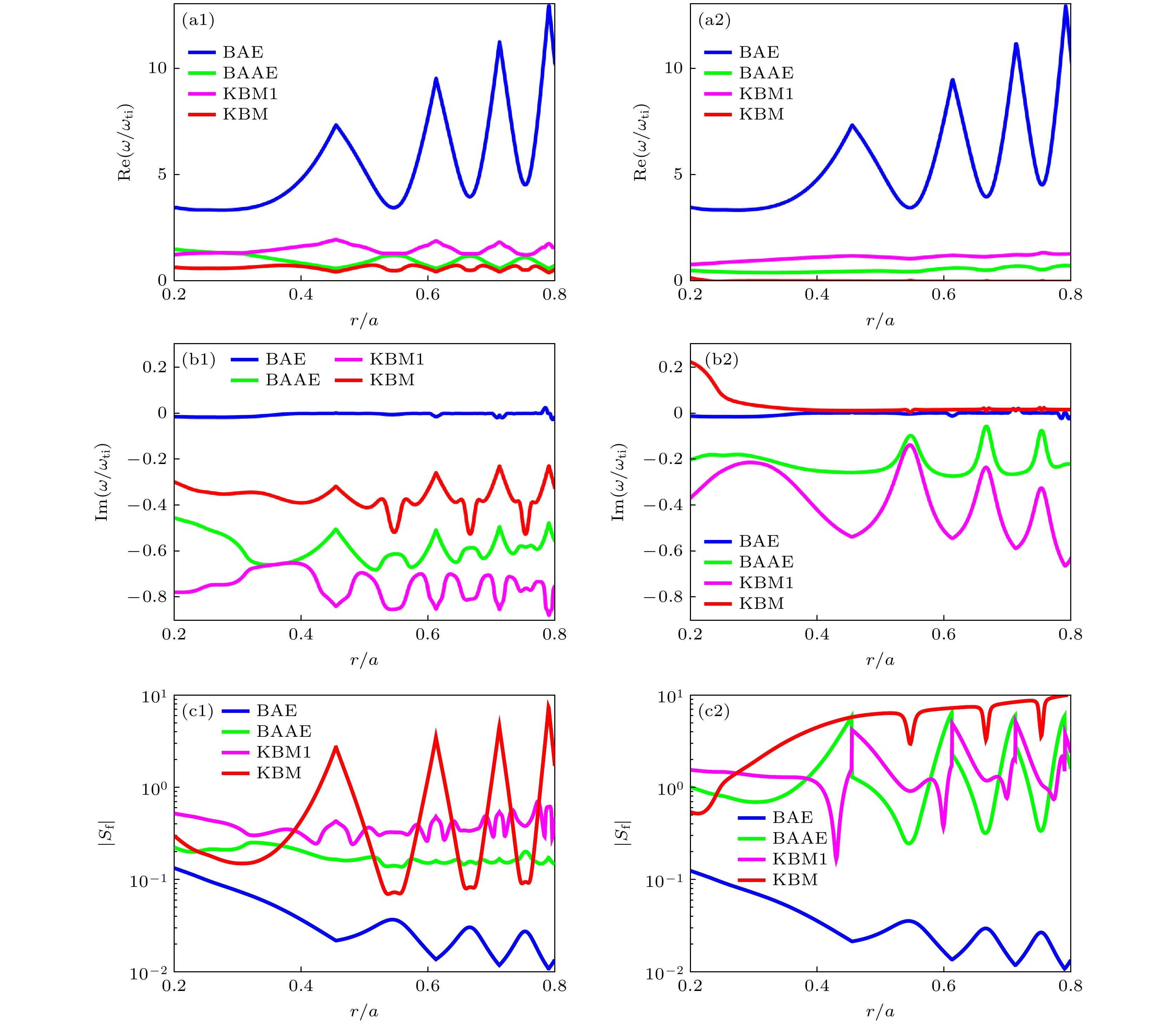
图 1 n = 3, m = 4—8的低频SAW和声波分支的连续谱, 此处采用了DIII-D第#178631次放电在1200 ms的平衡分布 (a1)—(c1)考虑了逆磁效应和热通行离子可压缩效应, 以及通过波-热离子相互作用和逆磁效应而产生的漂移阿尔芬波和漂移波边带模的耦合[7]的低频SAW连续谱; (a2)—(c2)包含了逆磁效应与热通行和热捕获离子的可压缩效应[5,8,28]
Fig. 1. Continuous spectra of low-frequency shear Alfvén and acoustic branches for n = 3, m = 4–8: (a1)–(c1) Considering the diamagnetic effects and thermal ion compressibility as well as drift Alfvén wave and drift wave sideband coupling via the wave-thermal-passing-ion interaction and diamagnetic effect[7]; (a2)–(c2) considering the diamagnetic effects and thermal ion compressibility (well passing and deeply trapped particle dynamics)[8,28]. The equilibrium profiles of DIII-D #178631 at 1200 ms are adopted
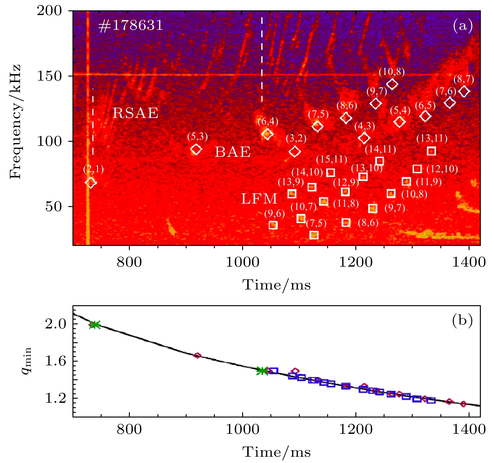
图 2 Heidbrink等[34]对DIII-D参考炮数#178631分析的实验结果 (a)布局在大半径R = 192—201 cm之间的ECE通道的互功率谱图; (b) EFIT重建得到的
$ q_{\min} $ 与时间的关系. 其中频谱图上所示的不同符号分别对应不同$ m/n $ 值的不同模式: RSAE($ \ast $ ), BAE($ \diamond $ )及LFAM($ \square $ )Fig. 2. The DIII-D experimental results from Ref. [34] by Heidbrink et al.: (a) Cross-power spectrogram in the reference shot for ECE channels between 192–201 cm; (b) measured
$ q_{\min} $ from EFIT reconstructions vs. time. The RSAE ($ \ast $ ), BAE($ \diamond $ ), and LFAM($ \square $ ) symbols represent the values of$ m/n $ shown on the spectrogram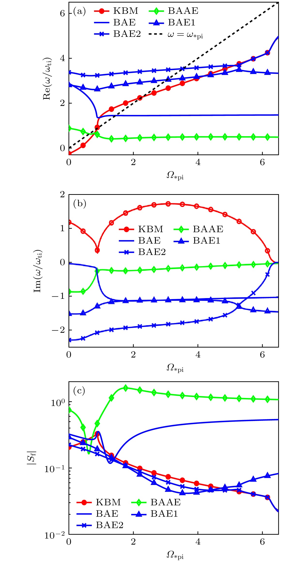
图 6 在不包含EP效应的情况下, 低频SAW的(a)频率、(b)增长率和(c)极化性质对
$ \varOmega_{\ast {\rm{pi}}}\equiv \omega_{\ast {\rm{pi}}}/\omega_{{\rm{ti}}} $ 的依赖关系Fig. 6. Dependence of (a) mode frequencies, (b) growth rates and (c) polarization of modes on
$ \varOmega_{\ast {\rm{pi}}}\equiv \omega_{\ast {\rm{pi}}}/\omega_{{\rm{ti}}} $ without EP effect.
图 3 热粒子和高能量粒子压强特征尺度(
$ L_{P_{\rm{th}}} $ 和$ L_{P_{\rm{E}}} $ ), 以及在弱和/或零磁剪切($ s=rq'/q $ )情况下模宽度($ {\varDelta}_m $ )的径向依赖关系Fig. 3. Radial dependences of the typical scale lengths of thermal and energetic particle pressure (
$ L_{P_{\rm{th}}} $ and$ L_{P_{\rm{E}}} $ ), magnetic shear (s) as well as the estimated radial mode width ($ {\varDelta}_m $ ).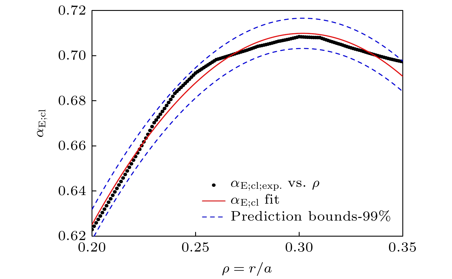
图 4 “经典”EP分布下EP归一化压强梯度的径向关系. 其中红线是解析拟合曲线,
$ q_{\min} $ 的归一化径向位置为$ \rho_0 $ $ \equiv r_0/a=0.28 $ Fig. 4. Radial dependence of the normalized pressure gradient of EPs with the classical profile. Here, the normalized radial position of
$ q_{\min} $ is$ \rho_0\equiv r_0/a=0.28 $ .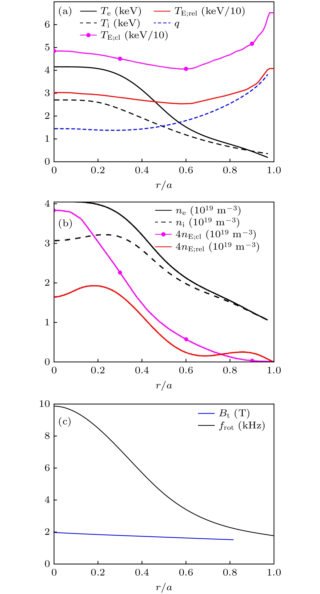
图 5 DIII-D第#178631次放电的(a)温度和q的径向分布, (b)密度的径向分布, 以及(c)环向磁场
$ B_{\rm{t}} $ 和环向旋转频率$ f_{{\rm{rot}}} $ 的径向分布Fig. 5. Radial profiles of (a) temperature and q, (b) density and (c)
$ B_{\rm{t}} $ as well as toroidal rotation frequency$ f_{{\rm{rot}}} $ of DIII-D shot #178631 used for numerical studies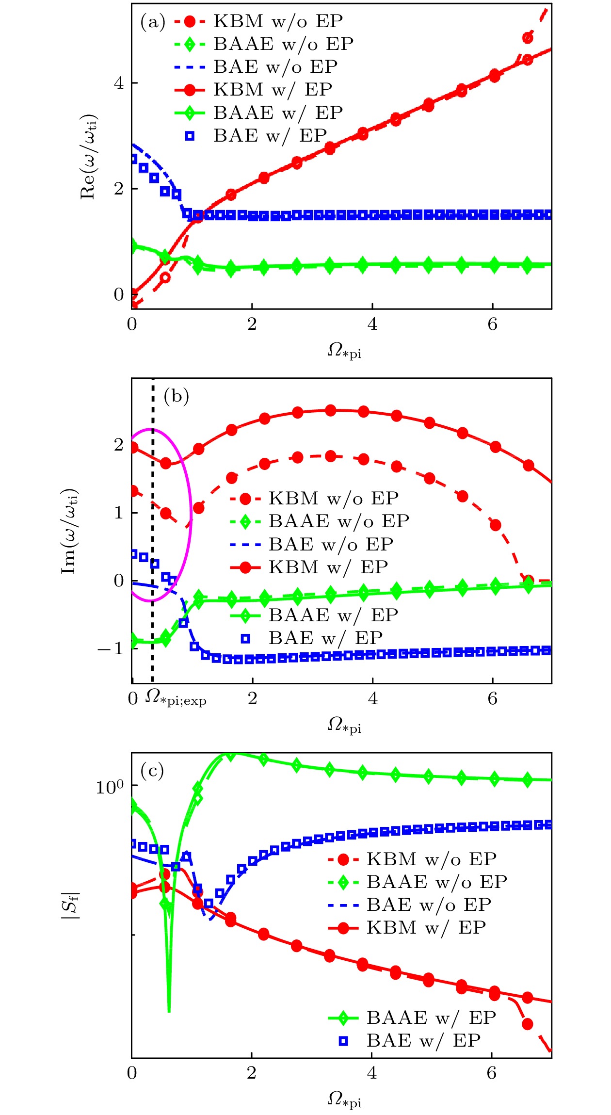
图 7 在不包含(w/o)和包含(w/)EP效应情况下, 低频SAW的(a)频率、(b)增长率和(c)极化性质对
$ \varOmega_{\ast {\rm{pi}}}\equiv $ $ \omega_{\ast {\rm{pi}}}/\omega_{{\rm{ti}}} $ 的依赖关系. 图中所示的垂直虚线表示$ \varOmega_{\ast{\rm{ pi}};{\rm{exp}}} $ 的实验值, 约为0.35Fig. 7. Dependence of the (a) real frequencies, (b) growth rates and (c) polarization of the low-frequency SAWs on
$ \varOmega_{\ast {\rm{p}}{\rm{i}}}\equiv \omega_{\ast {\rm{p}}{\rm{i}}}/\omega_{{\rm{ti}}} $ for the cases without (w/o) and with (w/) EP effects. Here, a dashed vertical line represents the experimental value of$ \varOmega_{\ast {\rm{pi}};{\rm{exp}}} $ of about 0.35
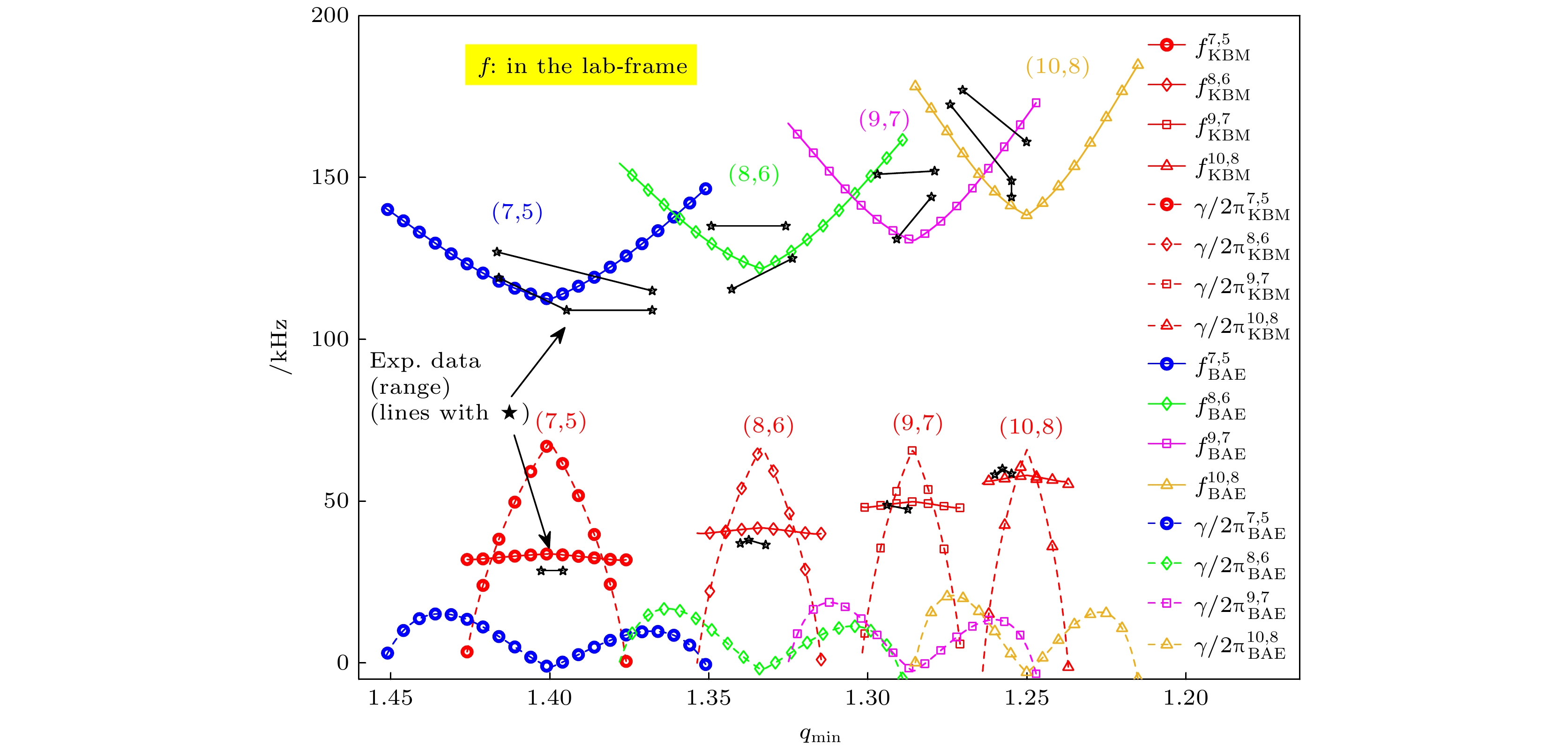
图 9 KBM (红色曲线)和BAE (蓝色、绿色、紫色和橙色曲线)的模频率(带标记的实线)和增长率(带标记的虚线)在不同(m, n)下对qmin的依赖关系. 图中还给出了实验观测的频率. 对于BAE, 由于模跨越了一个频率范围, 因此这些线表示不稳定区域的上下限; 对于LFAM, 实验频率变化小于0.5 kHz. 横坐标为
$ q_{\min} $ 的变化, 是依据参考文献[34]的图8所示的实验测量的$ q_{\min}(t) $ , 将时间t转换为$ q_{\min} $ 的变化, 与此相关的不确定度为$ \Delta q_{\min}\approx 0.01 $ . 纵坐标为理论实验室框架下的频率, 已将多普勒频移合并到计算的等离子体框架下的频率$ nf_{\rm rot} $ , 相关的不确定度为$ \sim0.5\times n $ kHzFig. 9. Dependence of mode frequencies (solid curves with markers) and growth rates (dashed curves with markers) on
$ q_{\min} $ of the KBMs (red curves) and the BAEs (blue, green, purple and orange curves) for different (m, n). The experimentally observed frequencies are also shown. For the BAE, since the modes span a range of frequencies, the lines indicate the upper and lower limits of the unstable bands; for the LFAM, the experimental frequency variation is$ <0.5 $ kHz. In the abscissa, the experimentally measured$ q_{\min}(t) $ fit shown in Fig. 8 of Ref. [34] is used to convert time to$ q_{\min} $ , with an associated uncertainty of$ \Delta q_{\min} \approx 0.01 $ . In the ordinate, the theoretical lab-frame frequency incorporates a Doppler shift to the calculated plasma-frame frequency of$ nf_{\rm rot} $ , with an associated uncertainty of$ \sim0.5\times n $ kHz.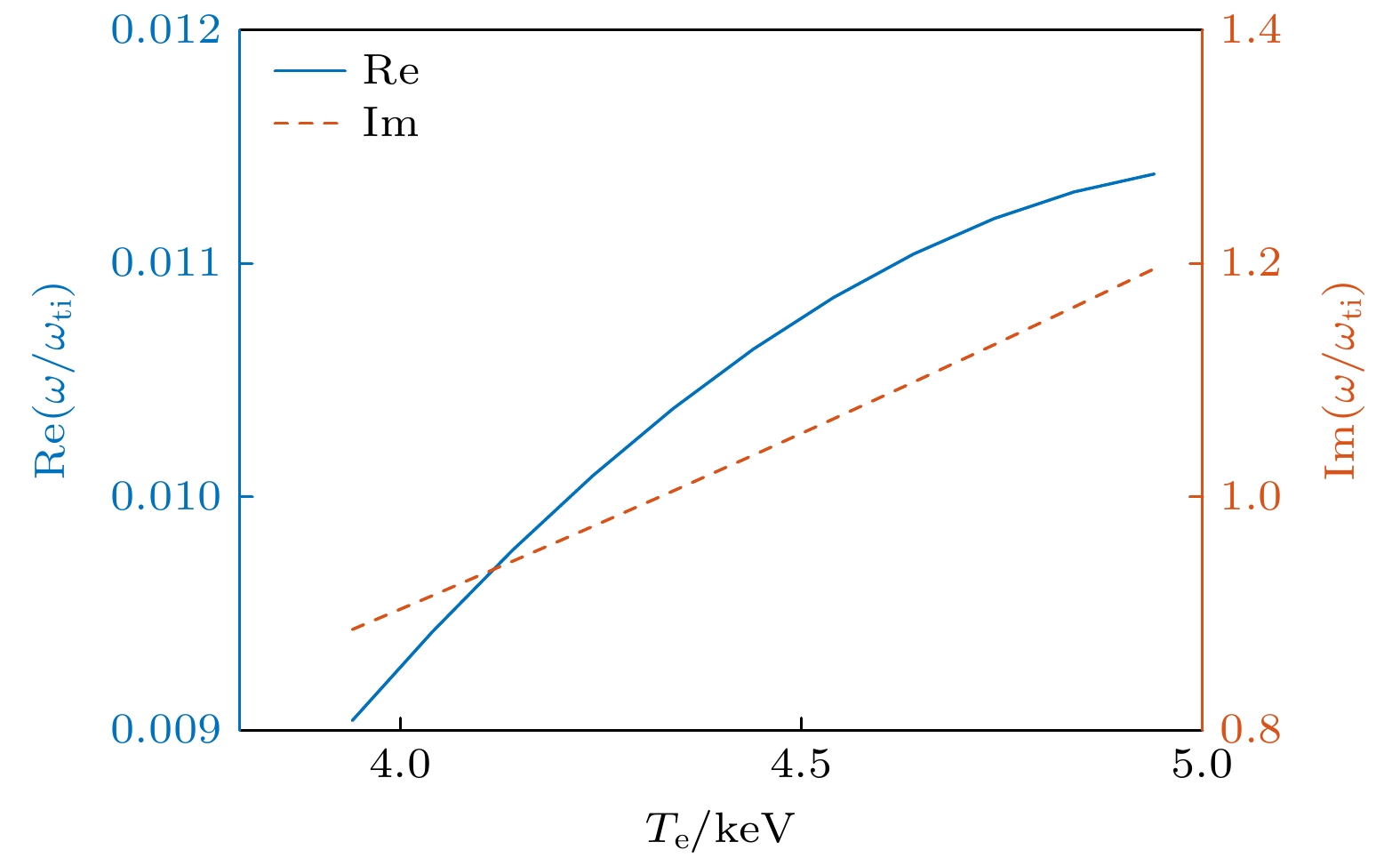
图 10 模频率(
$ {\rm{Re}}(\omega/\omega_{{\rm{ti}}}) $ )和增长率($ {\rm{Im}}(\omega/\omega_{{\rm{ti}}}) $ )对$ T_{\rm{e}} $ 的依赖关系, 其中$ T_{\rm{i}}=2.45 $ keVFig. 10. Dependence of mode frequency and growth rate on
$ T_{\rm{e}} $ . Here,$ T_{\rm{i}}=2.45 $ keV
图 11 KBM(三角形标记)和BAE(带标记的曲线)的频率(蓝色标记)和增长率(红色标记)与径向模数L的依赖关系
Fig. 11. Dependence of the real frequencies (blue markers) and growth rates (red markers) of the KBM (triangle markers) and BAE (line with markers) on the radial mode number L
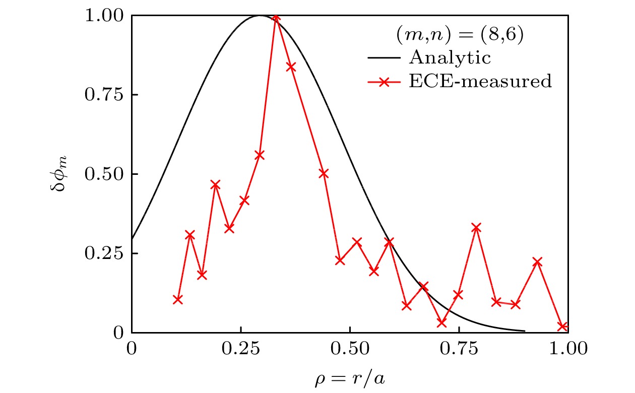
图 12
$ L=0 $ 的BAE的径向模结构$ {\text{δ}} \phi_{m} $ (r). 图中还给出了BAE模结构的近似实验测量结果, 如带‘$ \times $ ’的红线所示Fig. 12. Radial mode structure
$ {\text{δ}} \phi_{m} $ (r) for the$ L=0 $ BAE. The approximate experimental measurement of the mode structure of BAE is also shown.表 1 采用局域模型与全局模型计算(m, n) = (8, 6)低频SAW频率(
$ \omega/\omega_{{\rm{ti}}} $ )的对比Table 1. Comparison of the low-frequency SAW frequencies (
$ \omega/\omega_{{\rm{ti}}} $ ) with (m, n) = (8, 6) calculated by local and the global models模式 局域模型 全局模型 LFAM 0.224 + 0.704i –0.111 + 0.197i BAAE 0.824 – 0.908i 0.971 – 0.734i BAE 2.537 + 0.251i 2.807 + 0.527i  下载: 导出CSV
-
[1] Chen L, Zonca F 2016 Rev. Mod. Phys. 88 015008
Google Scholar
[2] Heidbrink W W, Strait E J, Chu M S, et al. 1993 Phys. Rev. Lett. 71 855
Google Scholar
[3] Turnbull A D, Strait E J, Heidbrink W W, et al. 1993 Phys. Fluids B 5 2546
Google Scholar
[4] Chen L, Zonca F 2007 Nucl. Fusion 47 S727
Google Scholar
[5] Zonca F, Chen L, Santoro R A 1996 Plasma Phys. Control. Fusion 38 2011
Google Scholar
[6] Zonca F, Chen L, Dong J Q, et al. 1999 Phys. Plasmas 6 1917
Google Scholar
[7] Zonca F, Biancalani A, Chavdarovski I, et al. 2010 J. Phys. Conf. Ser. 260 012022
Google Scholar
[8] Chavdarovski I, Zonca F 2009 Plasma Phys. Control. Fusion 51 115001
Google Scholar
[9] Lauber P, Brudgam M, Curran D, et al. 2009 Plasma Phys. Control. Fusion 51 124009
Google Scholar
[10] Zonca F, Chen L, Falessi M V, et al. 2021 J. Phys. Conf. Ser. 1785 012005
Google Scholar
[11] Cheng C 1982 Phys. Fluids 25 1020
Google Scholar
[12] Tang W, Connor J, Hastie R 1980 Nucl. Fusion 20 1439
Google Scholar
[13] Biglari H, Chen L 1991 Phys. Rev. Lett. 67 3681
Google Scholar
[14] Zonca F, Chen L, Botrugno A, et al. 2009 Nucl. Fusion 49 085009
Google Scholar
[15] Gorelenkov N, Berk H, Fredrickson E, et al. 2007 Phys. Lett. A 370 70
Google Scholar
[16] Gorelenkov N N, Zeeland M A V, Berk H L, et al. 2009 Phys. Plasmas 16 056107
Google Scholar
[17] Cheng C Z, Chen L, Chance M S 1985 Ann. Phys. 161 21
Google Scholar
[18] Kimura H, Kusama Y, Saigusa M, et al. 1998 Nucl. Fusion 38 1303
Google Scholar
[19] Sharapov S E, Testa D, Alper B, et al. 2001 Phys. Lett. A 289 127
Google Scholar
[20] Zonca F, Chen L 2014 Phys. Plasmas 21 072120
Google Scholar
[21] Zonca F, Chen L 2014 Phys. Plasmas 21 072121
Google Scholar
[22] Lu Z X, Zonca F, Cardinali A 2012 Phys. Plasmas 19 042104
Google Scholar
[23] Berk H L, Pfirsch D 1980 J. Math. Phys. 21 2054
Google Scholar
[24] Connor J, Hastie R, Taylor J 1979 Proc. R. Soc. London, Ser. A 365 1
Google Scholar
[25] Zonca F, Buratti P, Cardinali A, et al. 2007 Nucl. Fusion 47 1588
Google Scholar
[26] Chen W, Ding X T, Yang Q W, et al. 2010 Phys. Rev. Lett. 105 185004
Google Scholar
[27] Ma R, Qiu Z, Li Y, et al. 2021 Nucl. Fusion 61 036014
Google Scholar
[28] Chavdarovski I, Zonca F 2014 Phys. Plasmas 21 052506
Google Scholar
[29] Falessi M V, Carlevaro N, Fusco V, et al. 2019 Phys. Plasmas 26 082502
Google Scholar
[30] Falessi M V, Carlevaro N, Fusco V, et al. 2020 J. Plasma Phys. 86 845860501
Google Scholar
[31] Sharapov S, Alper B, Berk H, et al. 2013 Nucl. Fusion 53 104022
Google Scholar
[32] Gorelenkov N, Pinches S, Toi K 2014 Nucl. Fusion 54 125001
Google Scholar
[33] Heidbrink W, Zeeland M V, Austin M, et al. 2021 Nucl. Fusion 61 016029
Google Scholar
[34] Heidbrink W, Zeeland M V, Austin M, et al. 2021 Nucl. Fusion 61 066031
Google Scholar
[35] Heidbrink W, Choi G, Zeeland M V, et al. 2021 Nucl. Fusion 61 106021
Google Scholar
[36] Curran D, Lauber P, Carthy P J M, et al. 2012 Plasma Phys. Control. Fusion 54 055001
Google Scholar
[37] Lauber P 2013 Phys. Rep. 533 33
Google Scholar
[38] Fasoli A, Brunner S, Cooper W, et al. 2016 Nat. Phys. 12 411
Google Scholar
[39] Bierwage A, Lauber P 2017 Nucl. Fusion 57 116063
Google Scholar
[40] Choi G, Liu P, Wei X, et al. 2021 Nucl. Fusion 61 066007
Google Scholar
[41] Chen L, Hasegawa A 1991 J. Geophys. Res. 96 1503
Google Scholar
[42] Varela J, Spong D, Garcia L, et al. 2018 Nucl. Fusion 58 076017
Google Scholar
[43] Tsai S, Chen L 1993 Phys. Fluids B 5 3284
Google Scholar
[44] Chen L 1994 Phys. Plasmas 1 1519
Google Scholar
[45] Zonca F, Chen L 2000 Phys. Plasmas 7 4600
Google Scholar
[46] Zonca F, Briguglio S, Chen L, et al. 2002 Phys. Plasmas 9 4939
Google Scholar
[47] Ma R, Chen L, Zonca F, et al. 2022 Plasma Phys. Control. Fusion 64 035019
Google Scholar
[48] Ma R, Heidbrink W, Chen L, et al. 2023 Phy. Plasmas 30 042105
Google Scholar
[49] Lao L L, John H St, Stambaugh R D, et al. 1985 Nucl. Fusion 25 1611
Google Scholar
[50] Pankin A, McCune D, Andre R, et al. 2004 Comput. Phys. Commun. 159 157
Google Scholar
[51] Chen L, Zonca F 2017 Phys. Plasmas 24 072511
Google Scholar
[52] Connor J W, Hastie R J, Taylor J B 1978 Phys. Rev. Lett. 40 396
Google Scholar
[53] Chen L, White R B, Rosenbluth M 1984 Phys. Rev. Lett. 52 1122
Google Scholar
[54] Hasegawa A 1968 Phys. Rev. 169 204
Google Scholar
[55] O'Neil T, Malmberg J 1968 Phys. Fluids 11 1754
Google Scholar
[56] Rosenbluth M N, Hinton F L 1998 Phys. Rev. Lett. 80 724
Google Scholar
[57] Graves J P, Hastie R J, Hopcraft K I 2000 Plasma Phys. Control. Fusion 42 1049
Google Scholar


 下载:
下载:


计量
- 文章访问数: 6445
- PDF下载量: 116
- 被引次数: 0
