-
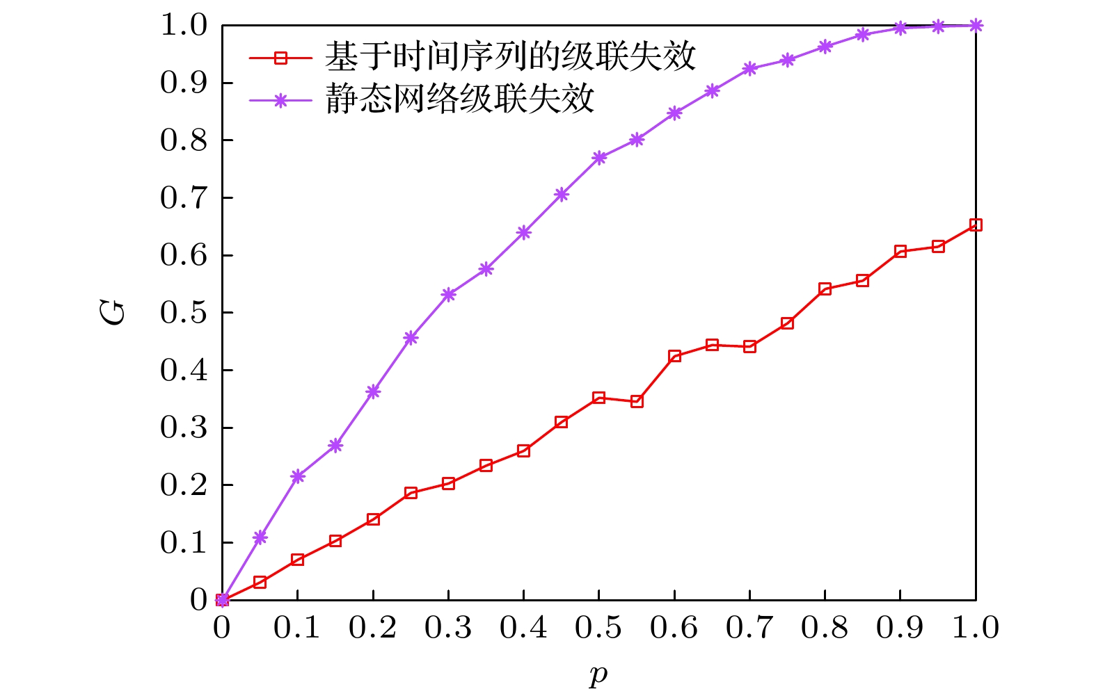
With the development of network science, the static network has been unable to clearly characterize the dynamic process of the network. In real networks, the interaction between individuals evolves rapidly over time. This network model closely links time to interaction process. Compared with static networks, dynamic networks can clearly describe the interaction time of nodes, which has more practical significance. Therefore, how to better describe the behavior changes of networks after being attacked based on time series is an important problem in the existing cascade failure research. In order to better answer this question, a failure model based on time series is proposed in this paper. The model is constructed according to time, activation ratio, number of edges and connection probability. By randomly attacking nodes at a certain time, the effects of four parameters on sequential networks are analyzed. In order to validate the validity and scientificity of this failure model, we use small social networks in the United States. The experimental results show that the model is feasible. The model takes into account the time as well as the spreading dynamics and provides a reference for explaining the dynamic networks in reality.
-
Keywords:
- time series /
- cascading failure /
- robustness
[1] Holme P 2003 Europhys. Lett. 64 427
 Google Scholar
[2] Holme P, Park S M, Kim B J, Edling C R 2007 Physica A 373 821
 Google Scholar
[3] Onody R N, Castro P A 2004 Phys. Rev. E 70 037103
 Google Scholar
[4] Albert R Jeong, H, Barabasi A 1999 Nature 401 130
 Google Scholar
[5] Perra N, Gonçalves B, Pastor R, Vespignani A 2012 Sci. Rep. 2 469
 Google Scholar
[6] Liao H, Mariani M S, Medo M, Zhang Y C 2017 Phys. Rep. 689 1
 Google Scholar
[7] Li A, Cornelius S, Liu Y Y, Wang L, Barabasi, A 2016 Science 358 1042
 Google Scholar
[8] Steven H 2001 Nature 401 268
 Google Scholar
[9] Remacle, Jean F, Flaherty, Joseph E, Shephard, Mark S 2003 SIAM Rev. 45 53
 Google Scholar
[10] 杨松青, 蒋沅, 童天驰, 严玉为, 淦各升 2021 物理学报 70 216401
 Google Scholar
Yang S Q, Jiang Y, Tong T C, Yan Y W, Gan G S 2021 Acta Phys. Sin. 70 216401
 Google Scholar
[11] Sole R V, Rosas M, Corominas B, Valverde S 2007 Phys. Rev. E 77 26102
 Google Scholar
[12] Goh K I, Kahng B, Kim D 2002 Phys. Rev. Lett. 88 108701
 Google Scholar
[13] Holme P, Kim B J, Yoon C N, Han S K 2002 Phys. Rev. E 65 056109
 Google Scholar
[14] Albert R, Jeong H, Barabasi A. L 2000 Nature 406 387
 Google Scholar
[15] Zhou T, Wang B H 2005 Chin. Phys. Lett. 22 1072
 Google Scholar
[16] Motter A E, Lai Y C 2003 Phys. Rev. E 66 065102
 Google Scholar
[17] Dou B L, Wang X G, Zhang S Y 2010 Physica A 389 2310
 Google Scholar
[18] Wang J 2012 Nonlinear Dyn. 70 1959
 Google Scholar
[19] Li S, Li L, Yang Y, Luo Q 2012 Nonlinear Dyn. 69 837
 Google Scholar
[20] Wang J, Rong L, Liang Z, Zhang Z 2008 Physica A 387 6671
 Google Scholar
[21] Liu J, Xiong Q Y, Shi X, Wang K, Shi W R 2015 Chin. Phys. B 24 371
 Google Scholar
[22] 唐亮, 焦鹏, 李纪康, 靖可, 靳志宏 2018 控制与决策 33 116
 Google Scholar
Tang L, Jiao P, Li J K, Jing K, Le Z H 2018 Control and Decision 33 116
 Google Scholar
[23] Duan D L, Ling X D, Wu X Y, Ouyang D H, Zhong B 2014 Physica A 2014 416 252
 Google Scholar
[24] 郝羽成, 李成兵, 魏磊 2018 系统工程与电子技术 40 2282
 Google Scholar
Hao Y C, Li C, Wei L 2018 Syst. Eng. Electron. 40 2282
 Google Scholar
-
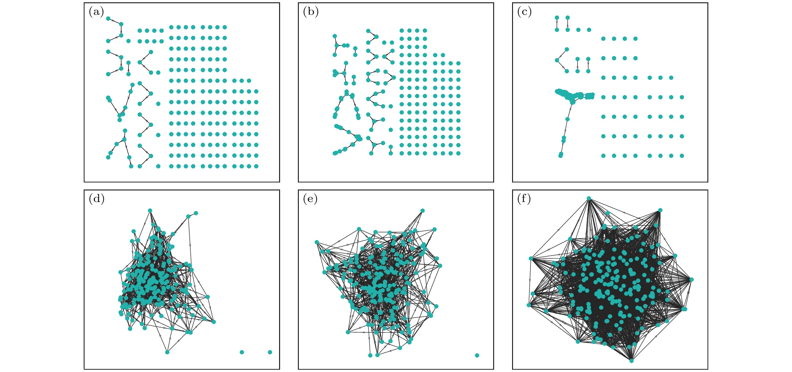
图 5 不同激活参数下的网络生成图 (a) pactive = 0.1; (b) pactive = 0.2; (c) pactive = 0.3; (d) pactive = 0.5; (e) pactive = 0.6; (f) pactive = 1.0
Figure 5. Network diagram with different activation parameters: (a) pactive = 0.1; (b) pactive = 0.2; (c) pactive = 0.3; (d) pactive = 0.5; (e) pactive = 0.6; (f) pactive = 1.0.
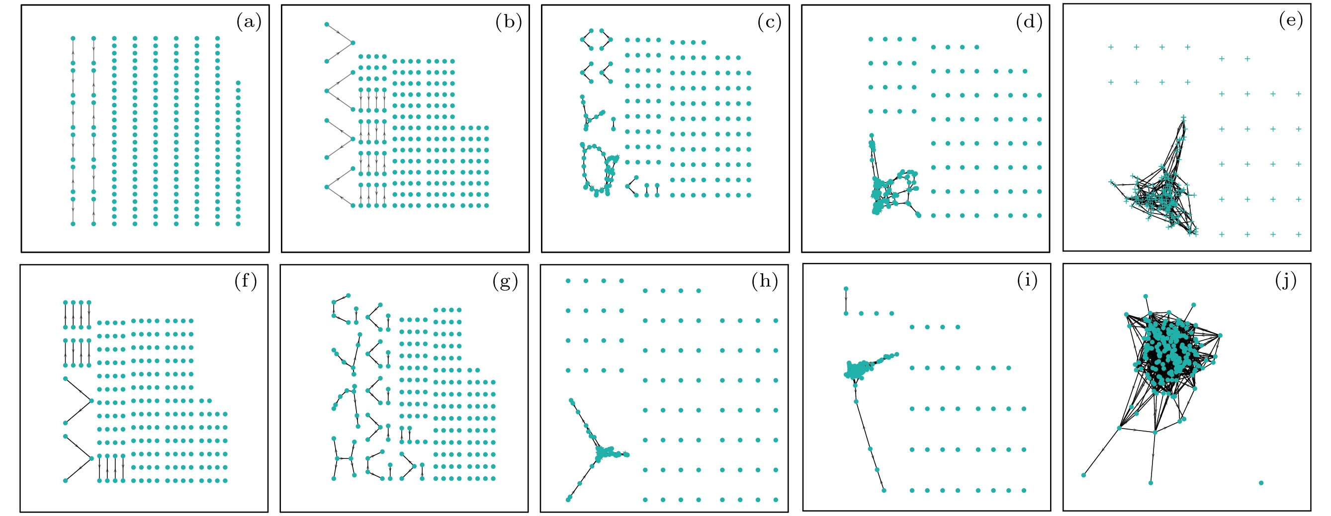
图 7 不同连接数以及连接概率下的网络生成图 (a) M = 1; (b) M = 2; (c) M = 5; (d) M = 8; (e) M = 10; (f) pcon = 0.1; (g) pcon = 0.2; (h) pcon = 0.5; (i) pcon = 0.6; (j) pcon = 1
Figure 7. Network diagram with different connection numbers and connection Probability: (a)M = 1; (b)M = 2; (c) M = 5; (d) M = 8; (e) M = 10; (f) pcon = 0.1; (g) pcon = 0.2; (h) pcon = 0.5; (i) pcon = 0.6; (j) pcon = 1.
表 1 激活参数下的网络特征
Table 1. Statistical characteristics of the networks under activation parameters.
pactive n m $\langle {k^{ { { {\rm{in} }/{\rm{out} } } } } } \rangle$ 0.1 200 32 0.16 0.2 200 68 0.34 0.3 200 191 0.955 0.5 200 787 3.945 0.6 200 843 4.215 1.0 200 3203 16.015 表 2 不同连接数以及连接概率下的网络特征
Table 2. Statistical characteristics of the networks under different connection numbers and connection probabilities.
Parameter n m $\langle {k^{ {\text{in} }/{\text{out} } } } \rangle$ M = 1 200 12 0.060 M = 2 200 24 0.120 M = 5 200 143 0.715 M = 8 200 507 2.535 M = 10 200 853 4.265 pcon = 0.1 200 16 0.080 pcon = 0.2 200 45 0.225 pcon = 0.5 200 179 0.895 pcon = 0.6 200 276 1.380 pcon = 1.0 200 983 4.915 表 3 不同时间下的网络特征
Table 3. Statistical characteristics of the networks under different time.
T n m $\langle {k^{ {\text{in} }/{\text{out} } } } \rangle$ 2 200 57 0.285 5 200 68 0.340 10 200 70 0.350 20 200 81 0.405 30 200 71 0.355 表 4 不同时间下的网络特征
Table 4. Statistical characteristics of the networks under different times.
T n m $\langle {k^{ {\text{in} }/{\text{out} } } } \rangle$ 2 200 931 4.655 5 200 5258 26.290 10 200 11689 58.445 20 200 15464 77.320 30 200 23062 115.310 表 5 美国小型社交网络的接触时刻
Table 5. Contact time of small social networks in the United States.
Source node Target node Time Source node Target node Time Source node Target node Time ${v_1}$ ${v_{12}}$ 4 ${v_3}$ ${v_{13}}$ 2 ${v_{16}}$ ${v_{10}}$ 2 ${v_1}$ ${v_{18}}$ 9 ${v_3}$ ${v_{18}}$ 2 ${v_{16}}$ ${v_{12}}$ 4 ${v_2}$ ${v_{10}}$ 7 ${v_3}$ ${v_{25}}$ 2 ${v_{16}}$ ${v_{14}}$ 2 ${v_2}$ ${v_{12}}$ 1 ${v_4}$ ${v_{10}}$ 4 ${v_{16}}$ ${v_{18}}$ 4 ${v_2}$ ${v_{13}}$ 1 ${v_4}$ ${v_{12}}$ 1 ${v_{16}}$ ${v_{32}}$ 1 ${v_2}$ ${v_{14}}$ 1 ${v_4}$ ${v_{27}}$ 1 ${v_{17}}$ ${v_{10}}$ 3 ${v_2}$ ${v_{18}}$ 1 ${v_4}$ ${v_{32}}$ 4 ${v_{18}}$ ${v_{12}}$ 2 ${v_3}$ ${v_{10}}$ 2 ${v_5}$ ${v_{12}}$ 4 ${v_{18}}$ ${v_{13}}$ 1 ${v_5}$ ${v_{13}}$ 1 ${v_8}$ ${v_{10}}$ 1 ${v_{18}}$ ${v_{14}}$ 2 ${v_5}$ ${v_{18}}$ 5 ${v_8}$ ${v_{12}}$ 2 ${v_{19}}$ ${v_{14}}$ 7 ${v_5}$ ${v_{20}}$ 1 ${v_8}$ ${v_{13}}$ 7 ${v_{21}}$ ${v_{13}}$ 1 ${v_5}$ ${v_{27}}$ 1 ${v_8}$ ${v_{15}}$ 1 ${v_{21}}$ ${v_{20}}$ 4 ${v_7}$ ${v_1}$ 1 ${v_8}$ ${v_{18}}$ 2 ${v_{22}}$ ${v_{10}}$ 3 ${v_7}$ ${v_{18}}$ 1 ${v_8}$ ${v_{20}}$ 2 ${v_{22}}$ ${v_{12}}$ 4 ${v_7}$ ${v_{33}}$ 1 ${v_8}$ ${v_{27}}$ 2 ${v_{22}}$ ${v_{13}}$ 1 ${v_8}$ ${v_2}$ 1 ${v_8}$ ${v_{32}}$ 2 ${v_{22}}$ ${v_{18}}$ 11 ${v_9}$ ${v_1}$ 3 ${v_{11}}$ ${v_{10}}$ 3 ${v_{22}}$ ${v_{27}}$ 3 ${v_9}$ ${v_5}$ 2 ${v_{11}}$ ${v_{12}}$ 1 ${v_{22}}$ ${v_{31}}$ 1 ${v_9}$ ${v_{12}}$ 1 ${v_{11}}$ ${v_{14}}$ 6 ${v_{24}}$ ${v_3}$ 2 ${v_9}$ ${v_{18}}$ 1 ${v_{11}}$ ${v_{18}}$ 1 ${v_{24}}$ ${v_6}$ 1 ${v_9}$ ${v_{33}}$ 2 ${v_{11}}$ ${v_{25}}$ 1 ${v_{24}}$ ${v_{10}}$ 8 ${v_{10}}$ ${v_{12}}$ 1 ${v_{11}}$ ${v_{30}}$ 3 ${v_{24}}$ ${v_{12}}$ 4 ${v_{10}}$ ${v_{13}}$ 1 ${v_{11}}$ ${v_{32}}$ 1 ${v_{24}}$ ${v_{13}}$ 3 ${v_{10}}$ ${v_{18}}$ 2 ${v_{16}}$ ${v_2}$ 1 ${v_{24}}$ ${v_{18}}$ 2 ${v_{24}}$ ${v_{25}}$ 3 ${v_{28}}$ ${v_5}$ 10 ${v_{33}}$ ${v_{10}}$ 2 ${v_{24}}$ ${v_{32}}$ 3 ${v_{28}}$ ${v_{12}}$ 2 ${v_{33}}$ ${v_{14}}$ 2 ${v_{24}}$ ${v_{33}}$ 1 ${v_{28}}$ ${v_{23}}$ 1 ${v_{33}}$ ${v_{25}}$ 1 ${v_{24}}$ ${v_{35}}$ 1 ${v_{29}}$ ${v_3}$ 1 ${v_{34}}$ ${v_{10}}$ 1 ${v_{25}}$ ${v_{10}}$ 1 ${v_{29}}$ ${v_{10}}$ 2 ${v_{34}}$ ${v_{12}}$ 9 ${v_{25}}$ ${v_{12}}$ 5 ${v_{29}}$ ${v_{12}}$ 6 ${v_{34}}$ ${v_{13}}$ 1 ${v_{25}}$ ${v_{14}}$ 4 ${v_{29}}$ ${v_{14}}$ 2 ${v_{34}}$ ${v_{14}}$ 1 ${v_{25}}$ ${v_{18}}$ 2 ${v_{29}}$ ${v_{15}}$ 2 ${v_{34}}$ ${v_{18}}$ 7 ${v_{26}}$ ${v_{10}}$ 3 ${v_{29}}$ ${v_{25}}$ 1 ${v_{34}}$ ${v_{20}}$ 2 ${v_{26}}$ ${v_{12}}$ 1 ${v_{29}}$ ${v_{32}}$ 4 ${v_{35}}$ ${v_2}$ 1 ${v_{26}}$ ${v_{14}}$ 12 ${v_{30}}$ ${v_{13}}$ 1 ${v_{35}}$ ${v_6}$ 1 ${v_{26}}$ ${v_{15}}$ 2 ${v_{30}}$ ${v_{14}}$ 7 ${v_{35}}$ ${v_{10}}$ 2 ${v_{26}}$ ${v_{18}}$ 1 ${v_{31}}$ ${v_{10}}$ 2 ${v_{35}}$ ${v_{12}}$ 2 ${v_{26}}$ ${v_{30}}$ 3 ${v_{31}}$ ${v_{13}}$ 3 ${v_{35}}$ ${v_{13}}$ 1 ${v_{35}}$ ${v_{14}}$ 4 ${v_{35}}$ ${v_{25}}$ 2 ${v_{35}}$ ${v_{32}}$ 3 ${v_{35}}$ ${v_{18}}$ 1 -
[1] Holme P 2003 Europhys. Lett. 64 427
 Google Scholar
[2] Holme P, Park S M, Kim B J, Edling C R 2007 Physica A 373 821
 Google Scholar
[3] Onody R N, Castro P A 2004 Phys. Rev. E 70 037103
 Google Scholar
[4] Albert R Jeong, H, Barabasi A 1999 Nature 401 130
 Google Scholar
[5] Perra N, Gonçalves B, Pastor R, Vespignani A 2012 Sci. Rep. 2 469
 Google Scholar
[6] Liao H, Mariani M S, Medo M, Zhang Y C 2017 Phys. Rep. 689 1
 Google Scholar
[7] Li A, Cornelius S, Liu Y Y, Wang L, Barabasi, A 2016 Science 358 1042
 Google Scholar
[8] Steven H 2001 Nature 401 268
 Google Scholar
[9] Remacle, Jean F, Flaherty, Joseph E, Shephard, Mark S 2003 SIAM Rev. 45 53
 Google Scholar
[10] 杨松青, 蒋沅, 童天驰, 严玉为, 淦各升 2021 物理学报 70 216401
 Google Scholar
Yang S Q, Jiang Y, Tong T C, Yan Y W, Gan G S 2021 Acta Phys. Sin. 70 216401
 Google Scholar
[11] Sole R V, Rosas M, Corominas B, Valverde S 2007 Phys. Rev. E 77 26102
 Google Scholar
[12] Goh K I, Kahng B, Kim D 2002 Phys. Rev. Lett. 88 108701
 Google Scholar
[13] Holme P, Kim B J, Yoon C N, Han S K 2002 Phys. Rev. E 65 056109
 Google Scholar
[14] Albert R, Jeong H, Barabasi A. L 2000 Nature 406 387
 Google Scholar
[15] Zhou T, Wang B H 2005 Chin. Phys. Lett. 22 1072
 Google Scholar
[16] Motter A E, Lai Y C 2003 Phys. Rev. E 66 065102
 Google Scholar
[17] Dou B L, Wang X G, Zhang S Y 2010 Physica A 389 2310
 Google Scholar
[18] Wang J 2012 Nonlinear Dyn. 70 1959
 Google Scholar
[19] Li S, Li L, Yang Y, Luo Q 2012 Nonlinear Dyn. 69 837
 Google Scholar
[20] Wang J, Rong L, Liang Z, Zhang Z 2008 Physica A 387 6671
 Google Scholar
[21] Liu J, Xiong Q Y, Shi X, Wang K, Shi W R 2015 Chin. Phys. B 24 371
 Google Scholar
[22] 唐亮, 焦鹏, 李纪康, 靖可, 靳志宏 2018 控制与决策 33 116
 Google Scholar
Tang L, Jiao P, Li J K, Jing K, Le Z H 2018 Control and Decision 33 116
 Google Scholar
[23] Duan D L, Ling X D, Wu X Y, Ouyang D H, Zhong B 2014 Physica A 2014 416 252
 Google Scholar
[24] 郝羽成, 李成兵, 魏磊 2018 系统工程与电子技术 40 2282
 Google Scholar
Hao Y C, Li C, Wei L 2018 Syst. Eng. Electron. 40 2282
 Google Scholar
Catalog
Metrics
- Abstract views: 7558
- PDF Downloads: 134
- Cited By: 0


 DownLoad:
