Search

Article

x

留言板

尊敬的读者、作者、审稿人, 关于本刊的投稿、审稿、编辑和出版的任何问题, 您可以本页添加留言。我们将尽快给您答复。谢谢您的支持!

姓名
邮箱
手机号码
标题
留言内容
验证码

Inversion models of internal solitary wave propagation speed in ocean based on least squares method and support vector machine

Liang Ke-Da Liu Teng-Fei Chang Zhe Zhang Meng Li Zhi-Xin Huang Song-Song Wang Jing

Liang Ke-Da, Liu Teng-Fei, Chang Zhe, Zhang Meng, Li Zhi-Xin, Huang Song-Song, Wang Jing. Inversion models of internal solitary wave propagation speed in ocean based on least squares method and support vector machine. Acta Phys. Sin., 2023, 72(2): 028301. doi: 10.7498/aps.72.20221633
Citation: Liang Ke-Da, Liu Teng-Fei, Chang Zhe, Zhang Meng, Li Zhi-Xin, Huang Song-Song, Wang Jing. Inversion models of internal solitary wave propagation speed in ocean based on least squares method and support vector machine. Acta Phys. Sin., 2023, 72(2): 028301. doi: 10.7498/aps.72.20221633

Inversion models of internal solitary wave propagation speed in ocean based on least squares method and support vector machine

Liang Ke-Da, Liu Teng-Fei, Chang Zhe, Zhang Meng, Li Zhi-Xin, Huang Song-Song, Wang Jing
Article Text (iFLYTEK Translation)
PDF
HTML
Get Citation
  • The propagation speed is one of the important parameters of the internal solitary wave (ISW). How to obtain the ISW speed through optical remote sensing images accurately and quickly is an important problem to be solved. In this paper, we simulate ISW optical remote sensing imaging, obtain an experimental database, and build the ISW speed inversion model based on a single-scene optical remote sensing image by using the least squares method and the support vector machine. The accuracy of the ISW speed inversion model is tested by using MODIS Image and GF-4 image data of the South China Sea. The study results are shown below. The least squares ISW speed inversion model can give the regression equation, which is more intuitive and has less accuracy in the water depth ranging from 300 m to 399 m, while the support vector machine ISW speed inversion model has high accuracy in the water depth ranging from 400 m to 1200 m and from 83 m to 299 m. Therefore, the two kinds of ISW speed inversion models have different advantages, and can be applied to the inversion of the ISW speed in the real ocean.
      PACS:
      83.60.Uv(Wave propagation, fracture, and crack healing)
      Corresponding author: Wang Jing, wjing@ouc.edu.cn
    • Funds: Project supported by the National Natural Science Foundation of China (Grant No. 61871353).

    为了满足日常生活中日益增长的储能需求, 人们需要探索具有高能量密度的新型动力电池[1]. 在各种后锂离子电池中, 如钠离子电池[24]、锂-硫电池[5]等, 能量密度高、成本低又环保的锂-氧电池被认为有希望成为锂离子电池的替代者[69]. 典型的锂-氧电池由空气阴极(活性氧)、高能量密度的锂金属阳极和高离子电导率的电解质组成, 通过简单的氧化还原反应2Li+O2Li2O2 (2.96 V vs Li/Li+)实现电池循环[10]. 锂-氧电池独特的反应使其能量密度超过3500Wh/kg, 远超最先进的锂离子电池和其他商用电池[11]. 对于典型的锂-氧电池, 充电-放电机理已经非常清楚, 固态过氧化锂被认为是反应的最终产物[12]. 放电过程, 金属锂氧化为Li+离子并释放电子, 氧气得到从外电路来的电子而被还原, 在阴极发生氧还原反应(ORR), 形成过氧化锂. 充电过程则相反, 过氧化锂被氧化, 释放氧气, 在阴极发生析氧反应(OER)[13]. 因此, 放电产物过氧化锂的形成和分解直接决定着锂-氧电池的循环性能[14].

    理论计算表明纯的过氧化锂是带隙为4.91 eV的绝缘体[15]. 绝缘性质限制了电子在过氧化锂里的迁移和电子从过氧化锂到阴极材料的转移, 导致锂-氧电池倍率性能下降[16]. 实际上, 过氧化锂由于其绝缘性很难被氧化, 氧化反应动能缓慢, 充电过电位高. 高过电位容易引起电解质和阴极材料不稳定等副反应[1719]. 因此, 为了提高锂-氧电池的能效和循环性能, 研究充电过程过氧化锂的氧化反应非常重要[20]. 为了提高过氧化锂氧化反应的动能, 人们设法提高阴极催化剂的催化活性. 在众多锂-氧电池阴极催化剂中, 如过渡金属氧化物MnO2[21,22]和Co3O4[2326]、贵金属Pt[27], Au[12,28]和Ru[29,30]等, 石墨烯基催化剂由于其比表面积大而备受关注[3133]. 研究发现石墨烯和N掺杂的石墨烯有很多活性电子, 可以作为锂-氧电池的ORR催化剂[3436]. 而对于OER, 过氧化锂需要转移电荷到催化剂表面氧化为氧气. 因此, B掺杂的石墨烯由于其p型行为有望作为过氧化锂OER的候选催化剂[37]. 而且, 实验上发现B原子可以掺杂到石墨烯的碳晶格位, 形成C=B共价键[37,38]. Ren等[39,40]研究表明硼掺杂石墨烯能够提高从过氧化锂到催化剂的电荷转移, 降低过氧化锂OER中的速率决定步势垒. 我们以前的研究发现硼掺杂石墨烯能够促进过氧化锂分子的氧化[41]. 另外, 相对于纯的石墨烯, 氧化石墨烯能够增强其与过氧化锂和超氧化锂分子的相互作用, 而且随着氧化浓度的升高, 从过氧化锂和超氧化锂分子向氧化石墨烯催化剂转移的电荷增加[32]. 更为重要的是在实际应用中, 纯的完美石墨烯很难制备, 常见的是氧化石墨烯或还原氧化石墨烯[30,42]. 因此, 本文利用第一性原理计算系统研究了B掺杂氧化石墨烯作为锂-氧电池阴极催化剂对过氧化锂OER的催化机理, 分析了B原子、O原子和C原子对过氧化锂氧化反应的协同催化作用.

    本工作利用第一性原理计算系统研究了硼掺杂氧化石墨烯的几何结构和电子性质, 对比研究了二聚体过氧化锂小团簇(Li2O2)2分别在氧化石墨烯和硼掺杂氧化石墨烯上的吸附结构、吸附强度和电荷转移, 对比分析了过氧化锂小团簇分别在氧化石墨烯和硼掺杂氧化石墨烯上的最优解离路径、吉布斯自由能、速率决定步和过电位. 结果发现B掺杂能大幅度提高从过氧化锂到催化剂的电荷转移, 而且在4电子氧化反应中, B掺杂能大大降低充电过电位.

    本文采用第一性原理计算软件VASP[43]完成, 离子实与价电子的相互作用采用投影缀加平面波描述[44], 电子与电子的交换关联采用广义梯度近似下的Perdew-Burke-Ernzerhof 泛函描述[45]. 石墨烯模型采用6×6×1的超胞, 包含72个碳原子, 晶格常数为 14.76 Å, 真空层为30 Å. 布里渊区积分采用Monkhorst-Pack型网格[46], k点取值为2×2×1. 态密度计算采用四面体展宽方法(ISMEAR = –5). 平面波基组展开的截止能量为520 eV, 力和总能量的收敛判据分别为0.02 eV/Å和10–4 eV/atom. 所有计算均考虑了自旋极化. 计算过氧化锂小团簇吸附时采用DFT-D3[47]方法修正范德瓦耳斯相互作用. 为了方便描述, 文章中氧化石墨烯用GO表示, 硼掺杂氧化石墨烯用BGO表示.

    图1给出了硼掺杂氧化石墨烯(BGO)的几何结构和电子性质. 为了对比, 图1同样给出了氧化石墨烯(GO)的几何结构和电子结构. 由图1(a)可以看出, 对于GO, 氧原子位于两个相邻碳原子的桥位, C—O键长1.467 Å, 局域氧化构型与文献[32,48]报道一致. 图1(c)显示GO打开了石墨烯的带隙(0.2 eV), C1与C2的电子态密度简并在一起. 在–1.0 eV附近及以下, O原子与C1和C2原子的电子态密度重叠. 图1(b)给出了硼掺杂氧化石墨烯的最低能量结构. 引入硼原子后, 氧原子位于碳原子和硼原子的桥位, 硼原子突出石墨烯表面与氧原子成键, B—O键长1.444 Å, C1—O键长1.395 Å, B—C2/C3键长1.510 Å. 图1(d)显示硼原子掺杂后, BGO的费米能级下移, 体系出现金属性质, 原因可能是硼原子比碳原子少电子, 硼原子替换碳原子, 使占据的电子态减少. 金属性说明BGO的电导率高, 更有利于电子传输, BGO更适合作为锂-氧电池阴极材料. 而且, C2与C3的电子态密度完全简并. 在–0.8 eV附近及以下, O原子与C1原子和B原子的电子态重叠, B原子还与C2/C3原子的电子态重叠. 更为重要的是, 在费米能级以下, 相比GO, 硼掺杂不仅增加了碳与硼对电子态的贡献, 还提高了氧的电子态密度, 这更有利于其与过氧化锂分子反应, 增强活性位点的催化活性. 另外, GO和BGO的电子态密度均为自旋非极化, 磁矩为零.

    图 1 氧化石墨烯和硼掺杂氧化石墨烯的几何结构和电子性质 (a), (b)几何结构, 灰色、红色和粉色小球分别代表C, O和B原子; (c), (d)电子性质, C1, C2和C3与结构图中相一致, 图中插入的是总态密度\r\nFig. 1. Geometric structure and electronic properties of oxide graphene (GO) and B doped oxide graphene (BGO): (a), (b) Geometric structures, grey, red and pink balls represent the C, O and B atoms, respectively; (c), (d) electronic properties, C1, C2 and C3 are consistent with those in the geometric structures, the insert is total density of states (TDOS).
    图 1  氧化石墨烯和硼掺杂氧化石墨烯的几何结构和电子性质 (a), (b)几何结构, 灰色、红色和粉色小球分别代表C, O和B原子; (c), (d)电子性质, C1, C2和C3与结构图中相一致, 图中插入的是总态密度
    Fig. 1.  Geometric structure and electronic properties of oxide graphene (GO) and B doped oxide graphene (BGO): (a), (b) Geometric structures, grey, red and pink balls represent the C, O and B atoms, respectively; (c), (d) electronic properties, C1, C2 and C3 are consistent with those in the geometric structures, the insert is total density of states (TDOS).

    为了进一步分析硼掺杂对氧化石墨烯电子结构的影响, 图2为硼掺杂前后氧化石墨烯的电荷密度差分和局域电子密度. 由图2可以看出氧原子获得电荷, 硼原子失去电荷. Bader电荷分析表明对于GO, C1与C2分别失去+0.33 e和+0.30 e, O原子得到–0.80 e. 对于BGO, C1失去+0.35 e, C2与C3分别得到–0.57 e和–0.56 e, B原子失去+1.97 e, O原子得到–1.24 e. 可见硼原子掺杂不仅使氧原子得到更多的电荷, 还使相邻的碳原子也得到电荷. 电子局域密度分析表明相对于GO, BGO的硼原子周围形成了缺电子活性中心, 这将有利于过氧化锂分子的吸附和解离.

    图 2 氧化石墨烯和硼掺杂氧化石墨烯的电荷密度差分和电子局域密度 (a), (b)电荷密度差分, 黄色和蓝色区域分别表示电荷聚积和电荷消失, 电荷等值面为0.004 e/Å3; (c), (d) 电子局域密度, 从红色到蓝色表示电子由多到少\r\nFig. 2. Charge density difference and electron localization function (ELF) of GO and BGO: (a), (b) Charge density difference, yellow and blue indicate the gain and the loss of electrons, and the isosurface value is 0.004 e/Å3; (c), (d) electron localization function, red to blue indicates more to less electrons.
    图 2  氧化石墨烯和硼掺杂氧化石墨烯的电荷密度差分和电子局域密度 (a), (b)电荷密度差分, 黄色和蓝色区域分别表示电荷聚积和电荷消失, 电荷等值面为0.004 e/Å3; (c), (d) 电子局域密度, 从红色到蓝色表示电子由多到少
    Fig. 2.  Charge density difference and electron localization function (ELF) of GO and BGO: (a), (b) Charge density difference, yellow and blue indicate the gain and the loss of electrons, and the isosurface value is 0.004 e/Å3; (c), (d) electron localization function, red to blue indicates more to less electrons.

    为了检验BGO对过氧化锂氧化反应的催化性能, 以二聚体过氧化锂小团簇(Li2O2)2作为过氧化锂模型, 计算了小团簇(Li2O2)2在BGO上的吸附性质, 如图3所示. 为了比较, 图3同样给出了小团簇(Li2O2)2在GO上的吸附性质. 结果显示小团簇(Li2O2)2在GO上吸附时有两个Li—O键形成, 而在BGO上吸附时有3个Li—O键形成. 另外, 小团簇(Li2O2)2在GO和BGO上的吸附能分别为1.08 eV和1.80 eV, 大的吸附能说明硼掺杂氧化石墨烯增强了与小团簇(Li2O2)2的相互作用, BGO更容易捕获过氧化锂团簇, 使过氧化锂氧化反应顺利进行. 另外, 放电产物过氧化锂与BGO的紧密结合使过氧化锂向阴极转移电子更容易, 更有利于降低电池的充电过电位. Bader电荷分析表明有0.59 e从(Li2O2)2团簇转移到GO, 而有0.96 e从(Li2O2)2团簇转移到BGO, 说明硼掺杂提高了从过氧化锂团簇到BGO的电荷注入, 有利于提高过氧化锂氧化反应的动能和降低充电过电位. 另外, 对于(Li2O2)2团簇在GO上吸附时, 团簇里的氧所带电荷(27.01 e)多于其在BGO上吸附时氧上所带电荷(26.64 e), 致使O—O键长大于其在BGO上吸附时的O—O键长. 以上这些分析都说明了BGO比GO更适合作为过氧化锂氧化反应的催化剂.

    图 3 (Li2O2)2团簇在氧化石墨烯(a)和硼掺杂氧化石墨烯(b)上吸附的俯视图和侧视图以及电荷转移, 箭头表示电荷转移方向, 青色和绿色分别代表(Li2O2)2团簇的O原子和Li原子\r\nFig. 3. Top view and side view of (Li2O2)2 cluster adsorbed on the GO (a) and BGO catalysts (b) along with the charge transfer, arrows indicate the direction of charge transfer. The cyan and green represent the O and Li atoms in the (Li2O2)2 cluster, respectively.
    图 3  (Li2O2)2团簇在氧化石墨烯(a)和硼掺杂氧化石墨烯(b)上吸附的俯视图和侧视图以及电荷转移, 箭头表示电荷转移方向, 青色和绿色分别代表(Li2O2)2团簇的O原子和Li原子
    Fig. 3.  Top view and side view of (Li2O2)2 cluster adsorbed on the GO (a) and BGO catalysts (b) along with the charge transfer, arrows indicate the direction of charge transfer. The cyan and green represent the O and Li atoms in the (Li2O2)2 cluster, respectively.

    为了进一步分析过氧化锂小团簇(Li2O2)2与GO和BGO的相互作用, 分别计算了(Li2O2)2团簇吸附之后的投影态密度, 如图4所示, O1和O2分别代表(Li2O2)2团簇中的O和催化剂上的O. 可以看出, 吸附了(Li2O2)2团簇之后, GO和BGO均为金属性质, 而且电子态密度出现了自旋极化. 另外, 在GO中, 出现了Li与O2的相互作用, 而在BGO中, 除了出现Li与O2的相互作用, 还出现B与O2的相互作用, 说明B与O对(Li2O2)2团簇起到了协同催化的作用.

    图 4 (Li2O2)2团簇在氧化石墨烯(a)和硼掺杂氧化石墨烯(b)上吸附的电子结构, 图中插入的是总态密度, O1和O2分别代表(Li2O2)2团簇和催化剂上的O\r\nFig. 4. Electronic structures of (Li2O2)2 cluster adsorbed on the GO (a) and BGO catalysts (b), the insert is TDOS. O1 and O2 represent O on (Li2O2)2 cluster and catalysts, respectively.
    图 4  (Li2O2)2团簇在氧化石墨烯(a)和硼掺杂氧化石墨烯(b)上吸附的电子结构, 图中插入的是总态密度, O1和O2分别代表(Li2O2)2团簇和催化剂上的O
    Fig. 4.  Electronic structures of (Li2O2)2 cluster adsorbed on the GO (a) and BGO catalysts (b), the insert is TDOS. O1 and O2 represent O on (Li2O2)2 cluster and catalysts, respectively.

    图5所示为(Li2O2)2小团簇在GO和BGO上按照Li-Li-O2路径解离的俯视图和侧视图及相应的吉布斯自由能. 为了更接近实际情况, 在计算中考虑了隐形溶剂四乙二醇二甲醚(TEGDME), 介电常数选为7.79[31]. 由图5可知, 采用Li-Li-O2解离路径, (Li2O2)2小团簇在GO和BGO上解离的速率决定步(RDS)均为第1步, 即Li4O4Li++e+Li3O4反应步. 另外, 在平衡电位下, (Li2O2)2小团簇在GO和BGO上解离的过电位分别是1.06 V和0.88 V. 因此, BGO降低了(Li2O2)2小团簇解离的过电位, 即降低了锂-氧电池的充电过电位. 因此, 可推测BGO作为锂-氧电池阴极催化剂更有助于放电产物的解离, 有效提高锂-氧电池的循环性能.

    图 5 (Li2O2)2团簇在GO (a)和BGO (b)上按照Li-Li-O2路径解离的俯视图和侧视图, 以及相应的吉布斯自由能曲线(c), (d)\r\nFig. 5. Top view and side view of (Li2O2)2 cluster dissociation on GO (a) and BGO (b) following the Li-Li-O2 pathway, and the corresponding Gibbs free energy profiles (c), (d).
    图 5  (Li2O2)2团簇在GO (a)和BGO (b)上按照Li-Li-O2路径解离的俯视图和侧视图, 以及相应的吉布斯自由能曲线(c), (d)
    Fig. 5.  Top view and side view of (Li2O2)2 cluster dissociation on GO (a) and BGO (b) following the Li-Li-O2 pathway, and the corresponding Gibbs free energy profiles (c), (d).

    接下来检查了Li-O2-Li解离路径. 图6(a), (b)分别显示了(Li2O2)2小团簇在GO和BGO上的解离过程, 图6(c), (d)分别显示了(Li2O2)2小团簇相应的解离吉布斯自由能. 可以看出, 在GO和BGO上, (Li2O2)2小团簇整个氧化反应的RDS均是解离第3个锂, 即Li2O2Li++e+LiO2反应步. 另外, 在平衡电位下, (Li2O2)2小团簇在GO和BGO上解离的过电位分别是0.76 V和0.23 V, 即BGO大大降低了锂-氧电池的充电过电位. 进一步检查RDS中Li2O2中间体的吸附能, 发现Li2O2分子在GO上的吸附能为1.68 eV, 而在BGO上的吸附能为1.58 eV. 反应中间体的吸附能减小有利于氧化反应的进行. 因此, Li2O2分子在BGO上的吸附能小于在GO上的吸附能, 说明Li2O2分子在BGO上更容易发生氧化反应. 最后, 与Li-Li-O2解离路径的过电位0.88 V相比, Li-O2-Li解离路径的过电位0.23 V更低, 说明Li-O2-Li是过氧化锂团簇最优的解离路径.

    图 6 (Li2O2)2团簇在GO (a)和BGO (b)上按照Li-O2-Li路径解离的俯视图和侧视图, 以及相应的吉布斯自由能曲线(c), (d)\r\nFig. 6. Top view and side view of (Li2O2)2 cluster dissociation on GO (a) and BGO (b) following the Li-O2-Li pathway, and the corresponding Gibbs free energy profiles (c), (d).
    图 6  (Li2O2)2团簇在GO (a)和BGO (b)上按照Li-O2-Li路径解离的俯视图和侧视图, 以及相应的吉布斯自由能曲线(c), (d)
    Fig. 6.  Top view and side view of (Li2O2)2 cluster dissociation on GO (a) and BGO (b) following the Li-O2-Li pathway, and the corresponding Gibbs free energy profiles (c), (d).

    本文通过第一性原理计算, 对比研究了氧化石墨烯和硼掺杂氧化石墨烯对过氧化锂小团簇氧化反应的催化机理. 结果表明, (Li2O2)2小团簇在GO和BGO上的吸附能分别为1.08 eV和1.80 eV, 从(Li2O2)2团簇转移到GO和BGO上的电荷分别为0.59 e和0.96 e, 可见B掺杂增强了与(Li2O2)2团簇的相互作用和电荷转移, 有利于提高锂-氧电池的反应动能, 降低充电过电位. 4电子分解过程的吉布斯自由能表明, (Li2O2)2团簇倾向于Li-O2-Li分解路径, GO和BGO的速率决定步均是第三步. 在平衡电位下, GO和BGO的充电过电位分别是0.76 V和0.23 V, 可见B掺杂大大降低了锂-氧电池的充电过电位. 电子态密度分析表明B掺杂调节了GO的电子结构, 增强了GO的电子电导, 并形成了缺电子活性中心, B与O对(Li2O2)2团簇起到了协同催化的作用.

    感谢合肥先进计算中心提供计算资源.

    [1]

    Yang Y C, Huang X D, Zhao W, Zhou C, Huang S W, Zhang Z W, Tian J W 2021 J. Phys. Oceanogr. 51 3609Google Scholar

    [2]

    关晖, 苏晓冰, 田俊杰 2011 计算力学学报 28 60Google Scholar

    Guan H, Su X B, Tian J W 2011 Chin. J. Comp. Mech. 28 60Google Scholar

    [3]

    刘国涛, 尚晓东, 陈桂英, 卢著敏, 刘良钢, 程晓波 2007 中山大学学报(自然科学版) 46 167Google Scholar

    Liu G T, Shang X D, Chen G Y, Lu Z M, Liu L G, Cheng X B 2007 Acta Sci. Natur. Univ. Sunyatseni 46 167Google Scholar

    [4]

    汪超, 杜伟, 杜鹏, 李卓越, 赵森, 胡海豹, 陈效鹏, 黄潇 2022 力学学报 54 1921Google Scholar

    Wang C, Du W, Du P, Li Z Y, Zhao S, Hu H B, Chen X P, Huang X 2022 Chin. J. Theor. App. Mech. 54 1921Google Scholar

    [5]

    汪超, 杜伟, 李广华, 杜鹏, 赵森, 李卓越, 陈效鹏, 胡海豹 2022 中国舰船研究 17 102Google Scholar

    Wang C, Du W, LI G H, Du P, Zhao S, Li Z Y, Chen X P, Hu H B 2022 Chin. J. Ship Res. 17 102Google Scholar

    [6]

    刘秀全, 陈国明, 畅元江, 姬景奇, 傅景杰, 张浩 2017 石油学报 38 1448Google Scholar

    Liu X Q, Chen G M, Chang Y J, Ji J Q, Fu J J, Zhang H 2017 Acta Petro. Sin. 38 1448Google Scholar

    [7]

    Farrar J T, Zappa C J, Weller R A, Jessup A T 2007 J. Geophys. Res-Oceans 112 1Google Scholar

    [8]

    蔡树群, 何建玲, 谢皆烁 2011 地球科学进展 26 703Google Scholar

    Cai S Q, He J L, Xie J H 2011 Adv. Earth Sci. 26 703Google Scholar

    [9]

    黄晓冬, 赵玮 2014 中国海洋大学学报(自然科学版) 44 19Google Scholar

    Huang X D, Zhao W 2014 Period. Ocean Univ. China 44 19Google Scholar

    [10]

    Cai S Q, Xie J S, He J L 2012 Surv. Geophys. 33 927Google Scholar

    [11]

    张涛, 张旭东 2020 海洋与湖沼 51 991Google Scholar

    Zhang T, Zhang X D 2020 Oceanologia Limnologia Sin. 51 991Google Scholar

    [12]

    邝芸艳, 王亚龙, 宋海斌, 关永贤, 范文豪, 龚屹, 张锟 2021 地球物理学报 64 597Google Scholar

    Kuang Y Y, Wang Y L, Song H B, Guan Y X, Fan W H, Ging Y, Zhang K 2021 Chin. J. Geophys. 64 597Google Scholar

    [13]

    孙丽娜, 张杰, 孟俊敏, 崔伟 2022 海洋学报 44 137Google Scholar

    Sun L N, Zhang J, Meng J M, Cui W 2022 Acta. Oceanol. Sin. 44 137Google Scholar

    [14]

    Alford M H, Lien R C, Simmons H, Klymak J, Ramp S, Yang Y J, Tang D, Chang M H 2010 J. Phys. Oceanogr. 40 1338Google Scholar

    [15]

    Huang X D, Chen Z H, Zhao W, Zhang Z W, Zhou C, Yang Q X, Tian J W 2016 Sci. Rep-UK. 6 30041Google Scholar

    [16]

    吕海滨, 何宜军, 申辉 2012 海洋科学 36 98Google Scholar

    LÜ H B, He Y J, Shen H 2012 Marine Sci. 36 98Google Scholar

    [17]

    Hong D B, Yang C S, Ouchi K 2015 Remote. Sens. Lett. 6 448Google Scholar

    [18]

    Meetei C, Nadimpalli J R, Dash M K, Barskar H 2020 Remote. Sens. Environ. 252 112123Google Scholar

    [19]

    Sun L N, Zhang J, Meng J M 2021 J. Oceanol. Limnol 39 14Google Scholar

    [20]

    Zhang M, Wang J, Li Z X, Liang K D, Chen X 2022 J. Geophys. Res-Oceans. 2 127Google Scholar

    [21]

    Wang J, Zhang M, Mei Y, Lu K X, Chen X 2020 IEEE. Geosci. Remote. S. 99 1Google Scholar

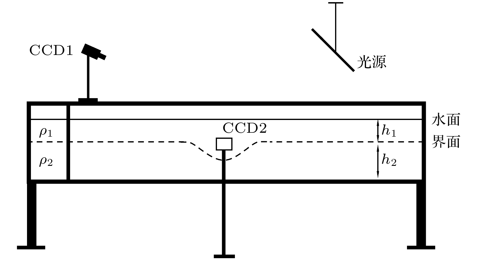
  • 图 1  内孤立波光学遥感仿真平台结构示意图

    Figure 1.  Schematic diagram of simulation platform of the internal solitary wave optical remote sensing.

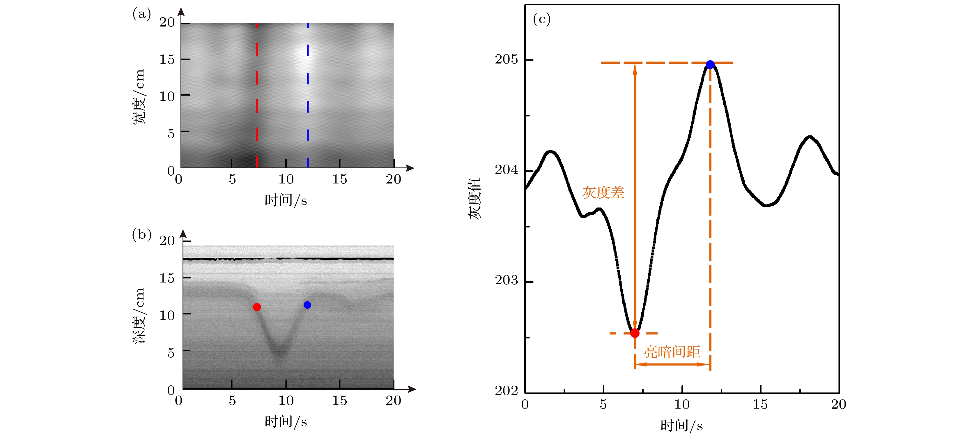
    图 2  实验室内孤立波参数示意图 (a) 内孤立波仿真遥感图像; (b)内孤立波波形图; (c)内孤立波灰度剖面图

    Figure 2.  Schematic diagram of the internal solitary wave parameters in the laboratory: (a) Simulated remote sensing images; (b) the internal solitary wave waveform diagram; (c) the gray scale profiles.

    图 3  最小二乘法回归方程反演结果散点图 (a)最高幂次为2次方; (b)最高幂次为3次方

    Figure 3.  Scatter plot of the inversion results of the least squares regression equation: (a) With the highest power of 2; (b) with the highest power of 3.

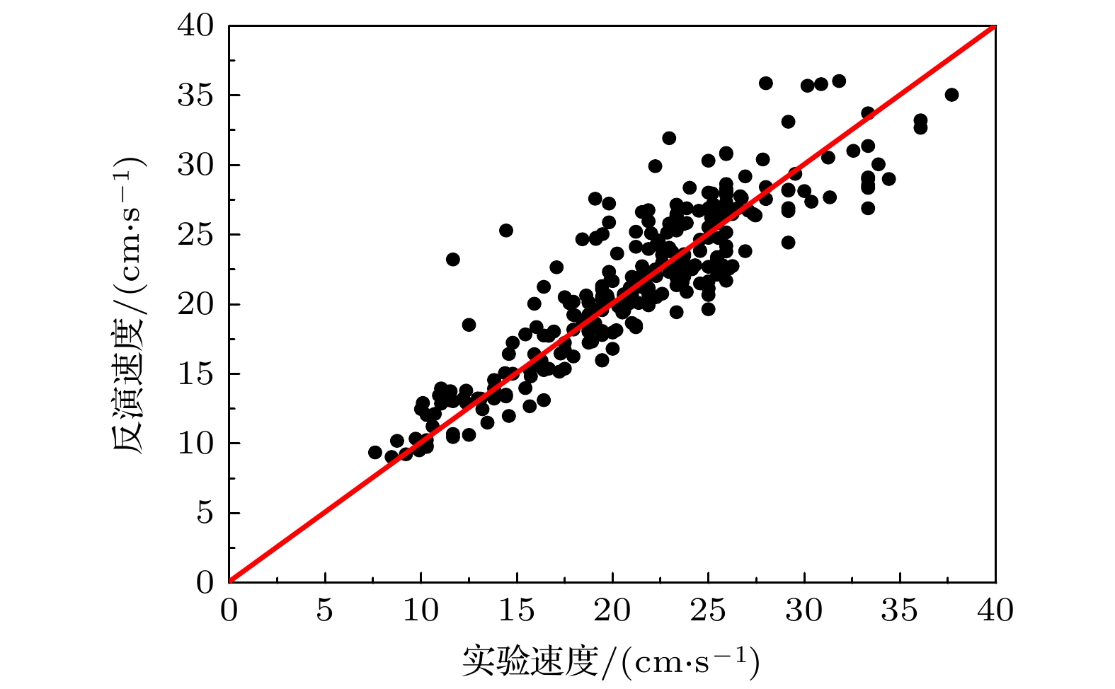
    图 4  SVR内孤立波速度反演模型测试集散点图

    Figure 4.  Scatter plot of test set of solitary wave speed inversion model in SVR.

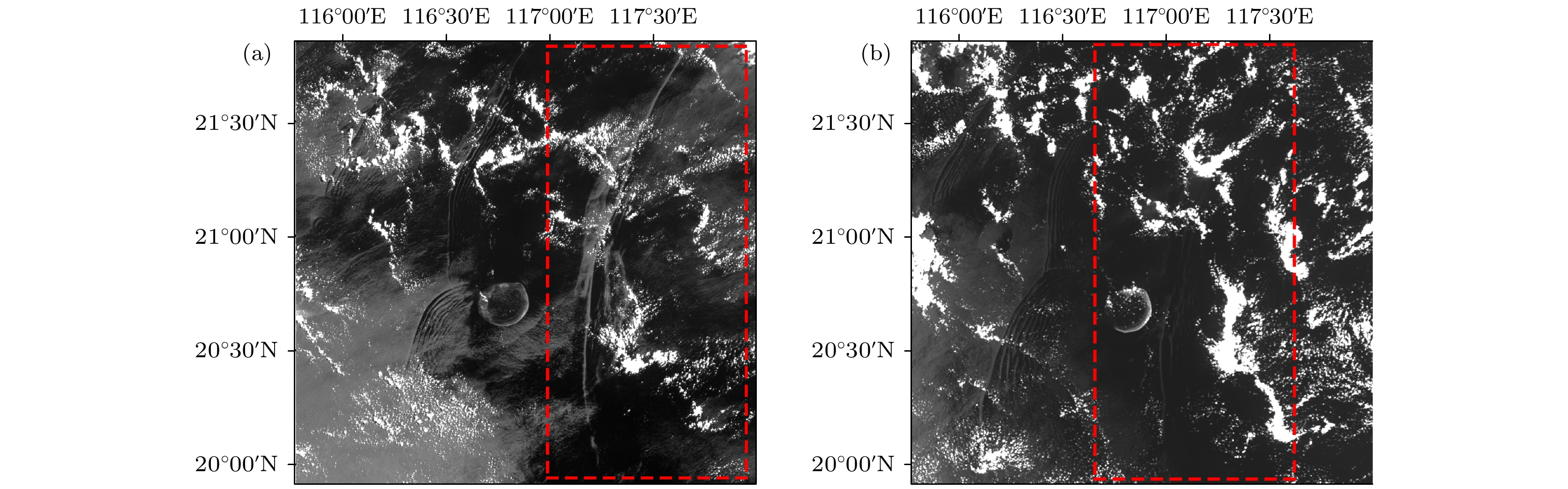
    图 5  多时间图像法示意图 (a) 2021年5月25日10:43 南海海域GF4光学遥感图像; (b) 2021年5月25日13:40南海海域 MODIS光学遥感图像

    Figure 5.  Schematic diagram of the multi-time image method: (a) An optical remote sensing image of GF-4 in the South China Sea at 10:43 on May 25, 2021; (b) the MODIS optical remote sensing image of the South China Sea area is at 13:40 on May 25, 2021.

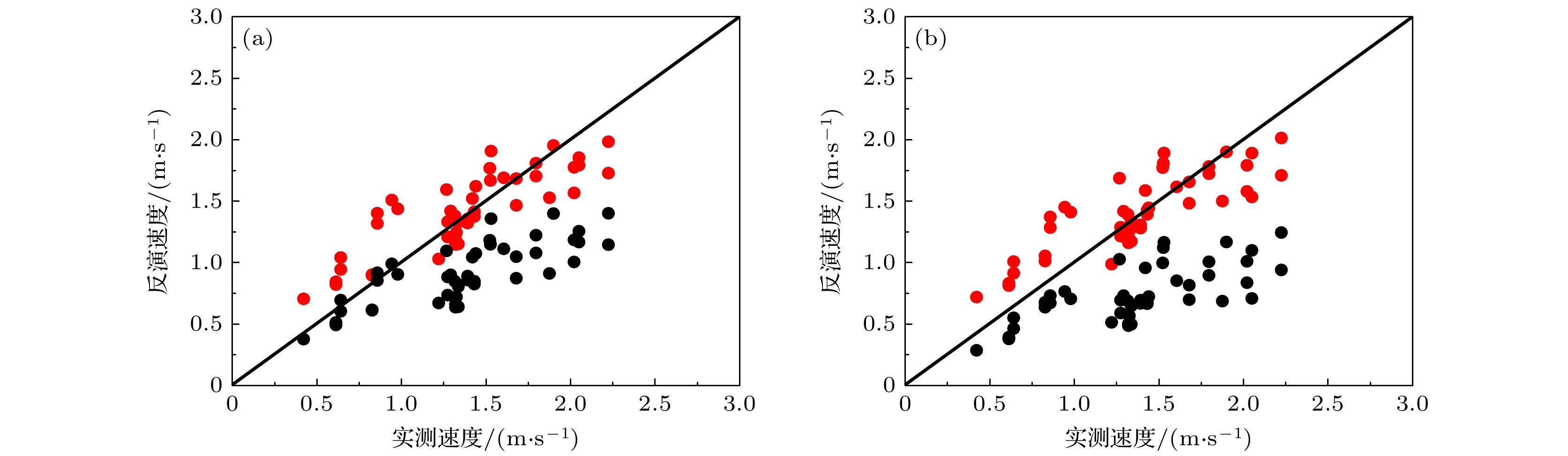
    图 6  最小二乘法内孤立波速度反演模型精度散点图 (a)校正前后最高幂次为2次方的最小二乘法回归方程的反演结果散点图, 黑色散点为校正前模型结果, 红色散点为校正后模型结果; (b)校正前后最高幂次为3次方的最小二乘法回归方程的反演结果散点图, 黑色散点为校正前模型结果, 红色散点为校正后模型结果.

    Figure 6.  Scatter plot of the solitary wave speed inversion model accuracy within least squares. (a) The scatter plot of inversion results of least squares regression equation with the highest power of 2 before and after correction. The black scatters are the model results before correction, and the red scatters are the model results after correction. (b) The scatter plot of the inversion results of the least squares regression equation with the highest power of 3 before and after correction. The black scatters are the model results before correction, and the red scatters are the model results after correction.

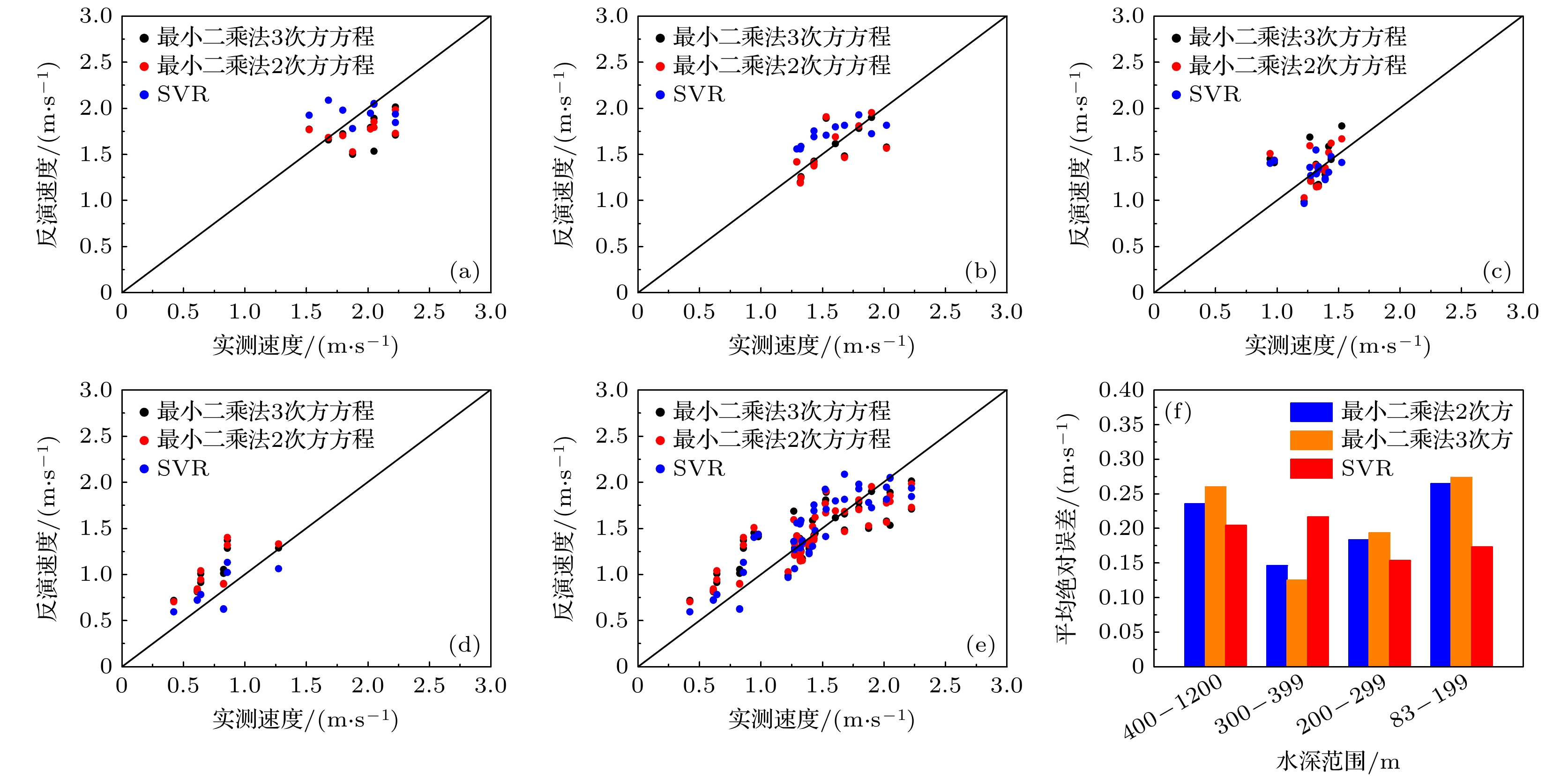
    图 7  内孤立波速度反演模型精度验证图 (a)—(d) 3种反演模型对400—1200 m、300—399 m、200—299 m、83—199 m水深范围的内孤立波的速度反演结果散点图; (e) 3种反演模型对83—1200 m水深范围的内孤立波的速度反演结果散点图; (a)—(e) 黑色散点为最高幂次为2次方的最小二乘法反演模型结果, 红色散点为最高幂次为3次方的最小二乘法反演模型结果, 蓝色散点为SVR反演模型结果; (f) 三种反演模型对400—1200 m、300—399 m、200—299 m、83—199 m水深范围的内孤立波的速度反演结果的平均绝对误差柱状图

    Figure 7.  Precision validation diagram of the internal solitary wave velocity inversion model: (a)–(d) Scatter plots of inversion results of three inversion models for internal solitary waves speed in water depths of 400–1200 m, 300–399 m, 200–299 m and 83–199 m, respectively; (e) scatter plot of inversion results of three inversion models for internal solitary waves speed in water depths of 83–1200 m; (a)–(e) the black scattered points are the results of least squares inversion model with the highest power of 2, the red scattered points are the results of least squares inversion model with the highest power of 3, and the blue scattered points are the results of SVR inversion model; (f) the average absolute error histogram of the inversion results of the three inversion models for internal solitary waves speed in the water depths of 400–1200 m, 300–399 m, 200–299 m and 83–199 m.

    表 1  内孤立波实验设计表

    Table 1.  Design table of internal solitary wave experiment.

    组数总水深/cm上层水深/cm下层水深/cm上层密度/(g·cm–3)下层密度/(g·cm–3)塌陷高度/cm
    1444401.001.085, 10, 15, 20
    2445391.001.085, 10, 15, 20
    34410341.001.085, 10, 15, 20
    44412321.001.085, 10, 15, 20
    5655601.001.045, 10, 15, 20
    6655601.011.045, 10, 15, 20
    7655601.021.045, 10, 15, 20
    86510551.001.045, 10, 15, 20, 25
    9688.559.51.001.045, 10, 15, 20
    10688.559.51.001.065, 10, 15, 20
    11688.559.51.001.085, 10, 15, 20
    DownLoad: CSV

    表 2  内孤立波速度反演模型精度验证表

    Table 2.  Precision verification table of internal solitary wave velocity inversion model.

    水深范围/m数据V/(m·s–1)VZ2/(m·s–1)AEz2/(m·s–1)VZ3/(m·s–1)AEz3(m·s–1)VSVR/(m·s–1)AESVR/(m·s–1)
    400—1200数据12.221.730.491.710.511.850.37
    数据22.051.850.201.890.162.040.01
    数据91.521.770.251.770.251.930.41
    300—399数据11.601.690.091.620.021.800.20
    数据21.901.950.051.9001.720.18
    数据111.431.380.051.390.041.690.26
    200—299数据11.321.380.061.390.071.550.23
    数据21.441.620.181.450.011.480.04
    数据141.221.030.190.990.230.970.25
    83—199数据10.861.400.541.370.511.130.27
    数据21.271.330.061.290.021.060.21
    数据100.830.900.071.010.180.620.21
    注: V表示遥感实测速度, VZ2表示最小二乘法二次方速度反演模型反演值, VZ3表示最小二乘法三次方速度反演模型反演值, VSVR表示SVR速度反演模型反演值, AEZ2表示VZ2V的绝对误差, AEZ3 表示VZ3V的绝对误差, AESVR表示VSVRV的绝对误差.
    DownLoad: CSV
  • [1]

    Yang Y C, Huang X D, Zhao W, Zhou C, Huang S W, Zhang Z W, Tian J W 2021 J. Phys. Oceanogr. 51 3609Google Scholar

    [2]

    关晖, 苏晓冰, 田俊杰 2011 计算力学学报 28 60Google Scholar

    Guan H, Su X B, Tian J W 2011 Chin. J. Comp. Mech. 28 60Google Scholar

    [3]

    刘国涛, 尚晓东, 陈桂英, 卢著敏, 刘良钢, 程晓波 2007 中山大学学报(自然科学版) 46 167Google Scholar

    Liu G T, Shang X D, Chen G Y, Lu Z M, Liu L G, Cheng X B 2007 Acta Sci. Natur. Univ. Sunyatseni 46 167Google Scholar

    [4]

    汪超, 杜伟, 杜鹏, 李卓越, 赵森, 胡海豹, 陈效鹏, 黄潇 2022 力学学报 54 1921Google Scholar

    Wang C, Du W, Du P, Li Z Y, Zhao S, Hu H B, Chen X P, Huang X 2022 Chin. J. Theor. App. Mech. 54 1921Google Scholar

    [5]

    汪超, 杜伟, 李广华, 杜鹏, 赵森, 李卓越, 陈效鹏, 胡海豹 2022 中国舰船研究 17 102Google Scholar

    Wang C, Du W, LI G H, Du P, Zhao S, Li Z Y, Chen X P, Hu H B 2022 Chin. J. Ship Res. 17 102Google Scholar

    [6]

    刘秀全, 陈国明, 畅元江, 姬景奇, 傅景杰, 张浩 2017 石油学报 38 1448Google Scholar

    Liu X Q, Chen G M, Chang Y J, Ji J Q, Fu J J, Zhang H 2017 Acta Petro. Sin. 38 1448Google Scholar

    [7]

    Farrar J T, Zappa C J, Weller R A, Jessup A T 2007 J. Geophys. Res-Oceans 112 1Google Scholar

    [8]

    蔡树群, 何建玲, 谢皆烁 2011 地球科学进展 26 703Google Scholar

    Cai S Q, He J L, Xie J H 2011 Adv. Earth Sci. 26 703Google Scholar

    [9]

    黄晓冬, 赵玮 2014 中国海洋大学学报(自然科学版) 44 19Google Scholar

    Huang X D, Zhao W 2014 Period. Ocean Univ. China 44 19Google Scholar

    [10]

    Cai S Q, Xie J S, He J L 2012 Surv. Geophys. 33 927Google Scholar

    [11]

    张涛, 张旭东 2020 海洋与湖沼 51 991Google Scholar

    Zhang T, Zhang X D 2020 Oceanologia Limnologia Sin. 51 991Google Scholar

    [12]

    邝芸艳, 王亚龙, 宋海斌, 关永贤, 范文豪, 龚屹, 张锟 2021 地球物理学报 64 597Google Scholar

    Kuang Y Y, Wang Y L, Song H B, Guan Y X, Fan W H, Ging Y, Zhang K 2021 Chin. J. Geophys. 64 597Google Scholar

    [13]

    孙丽娜, 张杰, 孟俊敏, 崔伟 2022 海洋学报 44 137Google Scholar

    Sun L N, Zhang J, Meng J M, Cui W 2022 Acta. Oceanol. Sin. 44 137Google Scholar

    [14]

    Alford M H, Lien R C, Simmons H, Klymak J, Ramp S, Yang Y J, Tang D, Chang M H 2010 J. Phys. Oceanogr. 40 1338Google Scholar

    [15]

    Huang X D, Chen Z H, Zhao W, Zhang Z W, Zhou C, Yang Q X, Tian J W 2016 Sci. Rep-UK. 6 30041Google Scholar

    [16]

    吕海滨, 何宜军, 申辉 2012 海洋科学 36 98Google Scholar

    LÜ H B, He Y J, Shen H 2012 Marine Sci. 36 98Google Scholar

    [17]

    Hong D B, Yang C S, Ouchi K 2015 Remote. Sens. Lett. 6 448Google Scholar

    [18]

    Meetei C, Nadimpalli J R, Dash M K, Barskar H 2020 Remote. Sens. Environ. 252 112123Google Scholar

    [19]

    Sun L N, Zhang J, Meng J M 2021 J. Oceanol. Limnol 39 14Google Scholar

    [20]

    Zhang M, Wang J, Li Z X, Liang K D, Chen X 2022 J. Geophys. Res-Oceans. 2 127Google Scholar

    [21]

    Wang J, Zhang M, Mei Y, Lu K X, Chen X 2020 IEEE. Geosci. Remote. S. 99 1Google Scholar

  • [1] Zhang Yi-Jun, Mu Xiao-Dong, Guo Le-Meng, Zhang Peng, Zhao Dao, Bai Wen-Hua. A support vector machine training scheme based on quantum circuits. Acta Physica Sinica, 2023, 72(7): 070302. doi: 10.7498/aps.72.20222003
    [2] Li Qin-Ran, Sun Chao, Xie Lei. Modal intensity fluctuation during dynamic propagation of internal solitary waves in shallow water. Acta Physica Sinica, 2022, 71(2): 024302. doi: 10.7498/aps.71.20211132
    [3] Zhi Chang-Hong, Xu Shuang-Dong, Han Pan-Pan, Chen Ke, You Yun-Xiang. Applicability of high-order unidirectional internal solitary wave theoretical model. Acta Physica Sinica, 2022, 71(17): 174701. doi: 10.7498/aps.71.20220411
    [4] Research on the modal intensity fluctuation during the dynamic propagation of internal solitary waves in the shallow water. Acta Physica Sinica, 2021, (): . doi: 10.7498/aps.70.20211132
    [5] Zhang Tao, Chen Wan-Zhong, Li Ming-Yang. Automatic seizure detection of electroencephalogram signals based on frequency slice wavelet transform and SVM. Acta Physica Sinica, 2016, 65(3): 038703. doi: 10.7498/aps.65.038703
    [6] Song Kun, Gao Tai-Chang, Liu Xi-Chuan, Yin Min, Xue Yang. Method and experiment of rainfall intensity inversion using a microwave link based on support vector machine. Acta Physica Sinica, 2015, 64(24): 244301. doi: 10.7498/aps.64.244301
    [7] Zhao Zhi-Gang, Zhang Chun-Jie, Gou Xiang-Feng, Sang Hu-Tang. Solar cell temperature prediction model of support vector machine optimized by particle swarm optimization algorithm. Acta Physica Sinica, 2015, 64(8): 088801. doi: 10.7498/aps.64.088801
    [8] Huang Wen-Hao, You Yun-Xiang, Wang Xu, Hu Tian-Qun. Wave-making experiments and theoretical models for internal solitary waves in a two-layer fluid of finite depth. Acta Physica Sinica, 2013, 62(8): 084705. doi: 10.7498/aps.62.084705
    [9] Zhao Yong-Ping, Zhang Li-Yan, Li De-Cai, Wang Li-Feng, Jiang Hong-Zhang. Chaotic time series prediction using filtering window based least squares support vector regression. Acta Physica Sinica, 2013, 62(12): 120511. doi: 10.7498/aps.62.120511
    [10] Du Hui, Wei Gang, Zhang Yuan-Ming, Xu Xiao-Hui. Experimental investigations on the propagation characteristics of internal solitary waves over a gentle slope. Acta Physica Sinica, 2013, 62(6): 064704. doi: 10.7498/aps.62.064704
    [11] Xing HongYan, Qi ZhengDong, Xu Wei. Weak signal estimation in chaotic clutter using selective support vector machine ensemble. Acta Physica Sinica, 2012, 61(24): 240504. doi: 10.7498/aps.61.240504
    [12] Wang Fang-Fang, Zhang Ye-Rong. An electromagnetic inverse scattering approach based on support vector machine. Acta Physica Sinica, 2012, 61(8): 084101. doi: 10.7498/aps.61.084101
    [13] Yan Xiao-Mei, Liu Ding. Control of fractional order chaotic system based on least square support vector machines. Acta Physica Sinica, 2010, 59(5): 3043-3048. doi: 10.7498/aps.59.3043
    [14] Prediction of chaotic time series based on selective support vector machine ensemble. Acta Physica Sinica, 2007, 56(12): 6820-6827. doi: 10.7498/aps.56.6820
    [15] Zhang Jia-Shu, Dang Jian-Liang, Li Heng-Chao. Local support vector machine prediction of spatiotemporal chaotic time series. Acta Physica Sinica, 2007, 56(1): 67-77. doi: 10.7498/aps.56.67
    [16] Ye Mei-Ying. Control of chaotic system based on least squares support vector machine modeling. Acta Physica Sinica, 2005, 54(1): 30-34. doi: 10.7498/aps.54.30
    [17] Ye Mei-Ying, Wang Xiao-Dong, Zhang Hao-Ran. Chaotic time series forecasting using online least squares support vector machine regression. Acta Physica Sinica, 2005, 54(6): 2568-2573. doi: 10.7498/aps.54.2568
    [18] Liu Han, Liu Ding, Ren Hai-Peng. Chaos control based on least square support vector machines. Acta Physica Sinica, 2005, 54(9): 4019-4025. doi: 10.7498/aps.54.4019
    [19] Cui Wan-Zhao, Zhu Chang-Chun, Bao Wen-Xing, Liu Jun-Hua. Prediction of the chaotic time series using support vector machines for fuzzy rule-based modeling. Acta Physica Sinica, 2005, 54(7): 3009-3018. doi: 10.7498/aps.54.3009
    [20] Cui Wan-Zhao, Zhu Chang-Chun, Bao Wen-Xing, Liu Jun-Hua. Prediction of the chaotic time series using support vector machines. Acta Physica Sinica, 2004, 53(10): 3303-3310. doi: 10.7498/aps.53.3303
Metrics
  • Abstract views:  5111
  • PDF Downloads:  65
Publishing process
  • Received Date:  16 August 2022
  • Accepted Date:  09 October 2022
  • Available Online:  01 November 2022
  • Published Online:  20 January 2023

/

返回文章
返回