


-
光参量啁啾脉冲放大(OPCPA)数值模拟平台研发涉及到光脉冲的展宽压缩、参量放大和聚焦输出等物理模型, 针对其中的超短脉冲聚焦算法, 本文推导给出了输出光场范围可调、并具备快速傅里叶算法的数学表达式, 解决了传统菲涅尔远场衍射聚焦算法面临如何提高光场分辨率和保持各波长分量计算网格大小一致的难题, 为后续直接进行时频逆变换、高效分析超短脉冲聚焦后的时空耦合特性提供了便利. 数值仿真结果揭示出, 超短脉冲聚焦场暗环区域表现出强烈的时空耦合特征. 本算法已成功应用于OPCPA数值仿真平台研发中, 可望在超短激光脉冲装置的优化设计工作中发挥重要作用.The development of optical parametric chirp pulse amplification (OPCPA) numerical simulation platform involves physical models such as broadening and compression of optical pulse, parametric amplification and focusing output. In the simulation platform, the Fresnel far-field diffraction equation is usually used to simulate the characteristics of ultrashort pulse focusing. Firstly, we need to calculate the optical field distribution of different wavelength components in the ultrashort pulse, and then use the inverse Fourier transform to obtain the temporal and spatial distribution characteristics of the pulse. However, for different wavelength components, the sizes of focused field grids obtained by the far-field algorithm are not equal, and subsequent resampling is required, which will increase the amount of calculation. In addition, due to the limitation of the calculation range of the light field in the pulse broadening and compression, there is also a problem of poor resolution of the focused field. In this work, the mathematical expression that can adjust the range of the output light field and use the fast fourier algorithm is derived. The main mechanism of this algorithm is as follows. Based on the Fresnel far-field diffraction equation, the output field is sampled independently in the discrete calculation process to meet the requirements for adjustable range of the output field. After identity transformation, the output field results can be calculated by the fast Fourier algorithm. Furthermore, the sampling conditions that need to be satisfied when using the algorithm are further analyzed and discussed. It solves the problem of how to improve the resolution of light field and keep the computational grid size of each wavelength component consistent when the traditional Fresnel far field diffraction is used to simulate the focusing process, which provides the convenience for the subsequent direct time-frequency inverse transformation. The numerical simulation results reveal that the dark ring region of the ultrashort pulse focusing field shows strong spatiotemporal coupling characteristics. This algorithm has been successfully applied to the development of OPCPA numerical simulation platform, and is expected to play an important role in optimizing the design of ultrashort laser pulse device.
-
Keywords:
- ultra-short pulse /
- focusing algorithm /
- spatial-temporal distribution /
- fast Fourier transform
[1] Wang D H, Shou Y R, Wang P J, Liu J B, Mei Z S, Cao Z X, Zhang J M, Yang P L, Feng G B, Chen S Y, Zhao Y Y, Joerg S, Ma W J 2020 High Power Laser Sci. 8 04000e41
 Google Scholar
[2] Danson C, Hillier D, Hopps N, Neely D 2015 High Power Laser Sci. 3 010000e3
Google Scholar
[3] Wang X B, Guang Y H, Zhang Z M, Gu Y Q, Zhao B, Zuo Y, Zheng J 2020 High Power Laser Sci. 8 04000e34
Google Scholar
[4] Zeng X M, Zhou K N, Zuo Y L, Zhu Q H, Su J Q, Wang X, Wang X D, Huang X J, Jiang X J, Jiang D B, Guo Y, Xie N, Zhou S, Wu Z H, Mu J, Peng H, Jing F 2017 Opt. Lett. 42 2014
Google Scholar
[5] Xiao Q, Pan X, Jiang Y E, Wang J F, Du L F, Guo J T, Huang D J, Lu X H, Cui Z J, Yang S S, Wei H, Wang X C, Xiao Z L, Li G Y, Wang X Q, Ouyang X P, Fan W, Li X C, Zhu J Q 2021 Opt. Express 29 15980
Google Scholar
[6] Begishev I A, Bagnoud V, Bahk S W, Bittle W A, Brent G, Cuffney R, Dorrer C, Froula D H, Haberberger D, Mileham C, Nilson P M, Okishev A V, Shaw J L, Shoup M J, Stillman C R, Stoeckl C, Turnbull D, Wager B, Zuegel J D, Bromage J 2021 Appl. Opt. 60 11104
Google Scholar
[7] 胡必龙, 王逍, 李伟, 曾小明, 母杰, 左言磊, 王晓东, 吴朝辉, 粟敬钦 2020 光学学报 40 222
Google Scholar
Hu B L, Wang X, Li W, Zeng X M, MU J, Zuo Y L, Wang X D, Wu C H, Su J Q 2020 Acta Opt. Sin. 40 222
Google Scholar
[8] 麦克斯 波恩, 埃米尔 沃尔夫著 (杨葭荪译) 2009 光学原理(第七版) (北京: 电子工业出版社) 第353—357页
Born M, Wolf E (translated by Yang J S) 2009 Principles of optics (7th Ed.) (Beijing: Electronic Industry Press) pp353–357 (in Chinese)
[9] 古德曼 J W (秦克诚, 刘培森, 陈家璧, 曹其智 译) 2016 傅里叶光学导论 (第三版) (北京: 电子工业出版社) 第46—49页
Goodman J W (translated by Qin K C, Liu P S, Chen J B, Cao Q Z) 2016 Introduction to Fourier Optics (3rd Ed.) (Beijing: Electronic Industry Press) pp46–49 (in Chinese)
[10] Talanov V I 1970 JETP Lett. 11 199
[11] Feigenbaum E, Sacks R A, McCandless K P, MacGowan B J 2013 Appl. Opt. 52 5030
Google Scholar
[12] Kozacki T, Falaggis K, Kujawinska M 2012 Appl. Opt. 51 7080
Google Scholar
[13] 杨美霞, 钟鸣, 任钢, 何衡湘, 刘文兵, 夏惠军, 薛亮平 2011 光学学报 31 72
Google Scholar
Yang M X, Zhong M, Ren G, He H X, Liu W B, Xia H J, Xue L P 2011 Acta Optic Sinica 31 72
Google Scholar
[14] Hu Y L, Wang Z Y, Wang X W, Ji S Y, Zhang C C, Li J W, Zhu W L, Wu D, Chu J R 2020 Light Sci. Appl. 9 119
Google Scholar
[15] Voelz D G 2010 Computational Fourier Optics (Bellingham: Washington SPIE Press) pp199−201
-

图 2 传统衍射算法聚焦光场分布 (a), (b)和(c)分别是波长λ = 0.74, 0.80和0.86 μm时的归一化二维强度分布; (d), (e)和(f)分别是波长λ = 0.74, 0.80 μm和0.86 μm时
${x'}$ 轴上归一化一维强度分布Fig. 2. Focusing light field distribution of traditional diffraction algorithm: (a), (b) and (c) The normalized two-dimensional intensity distribution at λ = 0.74, 0.80, and 0.86 μm, respectively; (d), (e) and (f) the normalized one-dimensional intensity distributions on the
${x'}$ axis at λ = 0.74, 0.80, and 0.86 μm, respectively.
图 3 本文算法聚焦光场分布 (a), (b)和(c)分别是波长λ = 0.74, 0.80和0.86 μm时的归一化二维强度分布; (d), (e)和(f)分别是波长λ = 0.74, 0.80和0.86 μm时
${x'}$ 轴上归一化一维强度分布Fig. 3. Focusing light field distribution of the proposed algorithm: (a), (b) and (c) The normalized two-dimensional intensity distribution at λ = 0.74, 0.80, and 0.86 μm, respectively; (d), (e) and (f) are the normalized one-dimensional intensity distributions on the
${x'}$ axis at λ = 0.74, 0.80, and 0.86 μm, respectively.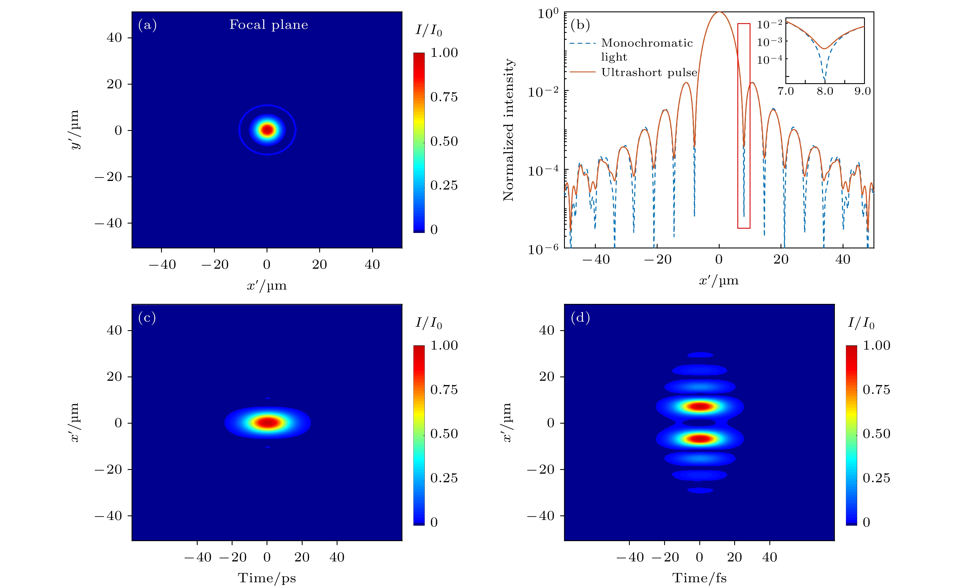
图 4 聚焦场的时空分布图 (a) 整体脉冲光的二维空间分布; (b)整体脉冲光和中心波长分量在
${x'}$ 轴上的一维分布对比(内插图为红色矩形方框范围内的放大图); (c)${y'} = 0{\kern 1 pt} {\kern 1 pt} {\kern 1 pt} {\text{μm}}$ 处的时空分布; (d)${y'} = 8.0{\kern 1 pt} {\kern 1 pt} {\kern 1 pt} {\kern 1 pt} {\text{μm}}$ 处的时空分布Fig. 4. Spatial-temporal distribution of the focused field: (a) The two-dimensional spatial distribution of the whole pulsed light; (b) one-dimensional distribution comparison of the whole pulse light and the central wavelength component on the
${x'}$ axis (the interpolation image is an enlarged image within the red rectangular box); (c) spatio-temporal distribution at${y'} = 0{\kern 1 pt} {\kern 1 pt} {\kern 1 pt} {\text{μm}}$ ; (d) spatio-temporal distribution at${y'} = 8.0{\kern 1 pt} {\kern 1 pt} {\kern 1 pt} {\kern 1 pt} {\text{μm}}$ .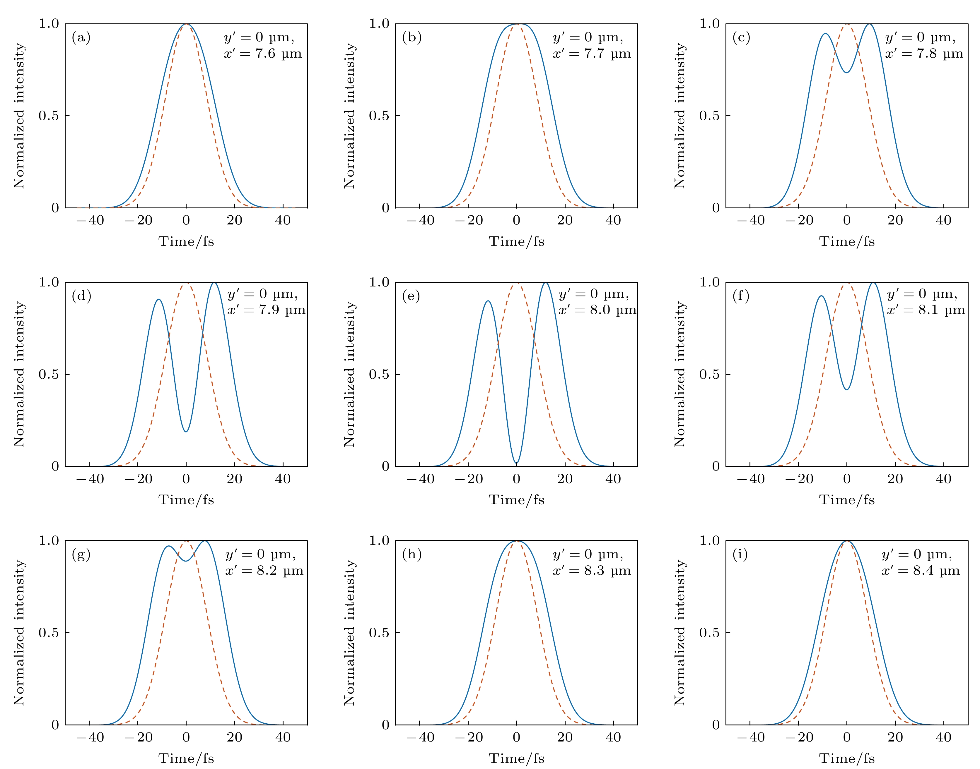
图 5 聚焦场
${x'}$ 轴上暗环附近时间波形演变图 (a)—(i)分别对应${x'}$ 轴上位置从7.6 μm以步长0.1 μm变化到8.4 μmFig. 5. Evolution of pulse shapes near the dark ring on
${x'}$ axis of focal field: (a)–(i) Corresponding to the axis position from 7.6 μm to 8.4 μm with a step of 0.1 μm.表 1 超短脉冲聚焦模拟计算参数
Table 1. Calculation parameters of ultrashort pulse focusing.
计算参数名称和符号/单位 参数数值 时域脉宽 ${\tau _{{\text{FWHM}}}}$/fs 20 中心波长 ${\lambda _0}$/μm 0.8 脉冲时间采样间隔 $\Delta t$/ fs 0.3 时域采样点数 ${N_{\text{t}}}$ 512 超高斯阶数 $n$ 12 输入光束半径 $R$/mm 50 输入光场采样点数 $N \times N$ $2048 \times 2048$ 输入光场采样间隔 $\text{δ} x$($\text{δ} y$)/mm 0.1 透镜后的传输距离 $z$/mm 800  下载: 导出CSV
-
[1] Wang D H, Shou Y R, Wang P J, Liu J B, Mei Z S, Cao Z X, Zhang J M, Yang P L, Feng G B, Chen S Y, Zhao Y Y, Joerg S, Ma W J 2020 High Power Laser Sci. 8 04000e41
Google Scholar
[2] Danson C, Hillier D, Hopps N, Neely D 2015 High Power Laser Sci. 3 010000e3
Google Scholar
[3] Wang X B, Guang Y H, Zhang Z M, Gu Y Q, Zhao B, Zuo Y, Zheng J 2020 High Power Laser Sci. 8 04000e34
Google Scholar
[4] Zeng X M, Zhou K N, Zuo Y L, Zhu Q H, Su J Q, Wang X, Wang X D, Huang X J, Jiang X J, Jiang D B, Guo Y, Xie N, Zhou S, Wu Z H, Mu J, Peng H, Jing F 2017 Opt. Lett. 42 2014
Google Scholar
[5] Xiao Q, Pan X, Jiang Y E, Wang J F, Du L F, Guo J T, Huang D J, Lu X H, Cui Z J, Yang S S, Wei H, Wang X C, Xiao Z L, Li G Y, Wang X Q, Ouyang X P, Fan W, Li X C, Zhu J Q 2021 Opt. Express 29 15980
Google Scholar
[6] Begishev I A, Bagnoud V, Bahk S W, Bittle W A, Brent G, Cuffney R, Dorrer C, Froula D H, Haberberger D, Mileham C, Nilson P M, Okishev A V, Shaw J L, Shoup M J, Stillman C R, Stoeckl C, Turnbull D, Wager B, Zuegel J D, Bromage J 2021 Appl. Opt. 60 11104
Google Scholar
[7] 胡必龙, 王逍, 李伟, 曾小明, 母杰, 左言磊, 王晓东, 吴朝辉, 粟敬钦 2020 光学学报 40 222
Google Scholar
Hu B L, Wang X, Li W, Zeng X M, MU J, Zuo Y L, Wang X D, Wu C H, Su J Q 2020 Acta Opt. Sin. 40 222
Google Scholar
[8] 麦克斯 波恩, 埃米尔 沃尔夫著 (杨葭荪译) 2009 光学原理(第七版) (北京: 电子工业出版社) 第353—357页
Born M, Wolf E (translated by Yang J S) 2009 Principles of optics (7th Ed.) (Beijing: Electronic Industry Press) pp353–357 (in Chinese)
[9] 古德曼 J W (秦克诚, 刘培森, 陈家璧, 曹其智 译) 2016 傅里叶光学导论 (第三版) (北京: 电子工业出版社) 第46—49页
Goodman J W (translated by Qin K C, Liu P S, Chen J B, Cao Q Z) 2016 Introduction to Fourier Optics (3rd Ed.) (Beijing: Electronic Industry Press) pp46–49 (in Chinese)
[10] Talanov V I 1970 JETP Lett. 11 199
[11] Feigenbaum E, Sacks R A, McCandless K P, MacGowan B J 2013 Appl. Opt. 52 5030
Google Scholar
[12] Kozacki T, Falaggis K, Kujawinska M 2012 Appl. Opt. 51 7080
Google Scholar
[13] 杨美霞, 钟鸣, 任钢, 何衡湘, 刘文兵, 夏惠军, 薛亮平 2011 光学学报 31 72
Google Scholar
Yang M X, Zhong M, Ren G, He H X, Liu W B, Xia H J, Xue L P 2011 Acta Optic Sinica 31 72
Google Scholar
[14] Hu Y L, Wang Z Y, Wang X W, Ji S Y, Zhang C C, Li J W, Zhu W L, Wu D, Chu J R 2020 Light Sci. Appl. 9 119
Google Scholar
[15] Voelz D G 2010 Computational Fourier Optics (Bellingham: Washington SPIE Press) pp199−201


 下载:
下载:


计量
- 文章访问数: 5670
- PDF下载量: 175
- 被引次数: 0
