


-
在大气压介质阻挡放电的某些应用场景中, 待处理物表面附着的水滴会改变气隙宽度、介电分布、气相成分等条件, 进而影响低温等离子体的应用效果. 本文建立了大气压氦气介质阻挡放电仿真模型, 探究了接触角为45°, 90°和135°的水滴附着于待处理物表面时稳态放电结构与活性粒子分布受到的影响及其背后机制. 结果表明, 水滴表面与上方区域的稳态放电强度受到削弱, 这是因为在负击穿中, 水滴表面的极化电场增强了等离子体双极性扩散, 促成环形放电抑制区; 在次正放电阶段, 水滴极化导致的种子电子清除效应抑制了水滴上方区域放电, 上述放电抑制作用随水滴接触角变大而提升. 在化学分布部分, 待处理物和水滴表面的活性粒子与电子存在着协同分布关系, 其中O与N的分布会因O2与N2键能的不同产生差异, OH与He+的分布则分别受到水滴蒸发与电场的影响. 本文系统地阐述了水滴附着对介质阻挡放电电化学过程的影响机制, 为等离子体-液滴系统的相关应用提供了理论指导.Dielectric barrier discharge technology can generate cold plasma at atmospheric pressure, which contains abundant active particles and shows great potential for fresh produce sterilization applications. However, water droplets frequently adhere to the surfaces of fruits and vegetables, which changes key parameters including the gas gap width, dielectric distribution, and gas-phase composition, consequently affecting the effectiveness of plasma applications. Currently, plasma-droplet interactions with contact angle as a variable remain unexplored, and the underlying mechanisms by which adhering droplets affect the electrochemical characteristics of dielectric barrier discharge require further investigation. In this work, we develop an atmospheric-pressure helium dielectric barrier discharge simulation model with an He-O2-N2-H2O reaction system. This model is used to study how water droplets (with contact angles of 45°, 90°, and 135°) adhering to the surface of the specimens affect both the steady-state discharge structure and active particle distribution, as well as their underlying mechanisms. The results show that the steady-state discharge intensity is significantly weakened both at the droplet surface and in the region above it, with the greatest reduction occurring at a contact angle of 135°. During the main positive breakdown phase, the polarized electric field at the droplet surface significantly enhances both electron impact ionization and secondary electron emission, thereby promoting gas-phase breakdown in the region above the water droplet. During the main negative breakdown phase, this polarized electric field accelerates electron migration toward the liquid surface, which intensifies plasma ambipolar diffusion and consequently leads to the formation of an annular discharge suppression zone around the water droplet. During the secondary positive discharge phase, even though the water droplet becomes polarized and a radially inward electric field is generated near the liquid surface, the resulting seed electron scavenging effect suppresses discharge in the region above the water droplet. Due to the stronger polarized electric fields generated at the surfaces of water droplets with larger contact angles, both the discharge enhancement and suppression effects become more pronounced with the increase of contact angle. Regarding the chemical species distribution, active particles and electrons exhibit a synergistic distribution relationship. On the surface of the specimens, He+ ions undergo electric field-driven migration, resulting in a highly non-uniform spatial distribution. The evaporation of water droplets provides more reactant sources for OH generation, thereby increasing its total deposition quantity. Because the bond energy of O2 is lower than that of N2, oxygen (O) demonstrates a more uniform distribution and a greater total deposition quantity than nitrogen (N). On the surfaces of water droplets, the active particles exhibit a gradually decreasing distribution from the center to the edge. Notably, the total deposition quantity of He+ continuously increases with larger contact angles increasing due to the aggregation effect of the polarized electric field. This study systematically elucidates the influence mechanisms of adhering water droplets on the electrochemical processes in dielectric barrier discharge, providing theoretical guidance for relevant applications of plasma-droplet systems.
-
Keywords:
- dielectric barrier discharge /
- water droplet /
- discharge structure /
- active particle
[1] Zhang S, Oehrlein G S 2021 J. Phys. D: Appl. Phys. 54 213001
 Google Scholar
[2] Chen Z T, Chen G J, Obenchain R, Zhang R, Bai F, Fang T X, Wang H W, Lu Y J, Wirz R E, Gu Z 2022 Mater. Today 54 153
Google Scholar
[3] Poggemann H-F, Schüttler S, Schöne A L, Jeß E, Schücke L, Jacob T, Gibson A R, Golda J, Jung C 2025 J. Phys. D: Appl. Phys. 58 135208
Google Scholar
[4] Zhou B S, Zhao H G, Yang X, Cheng J-H 2024 Food Res. Int. 196 115117
Google Scholar
[5] Woedtke T, Laroussi M, Gherardi M 2022 Plasma Sources Sci. Technol. 31 054002
Google Scholar
[6] Moldgy A, Nayak G, Aboubakr H A, Goyal S M, Bruggeman P J 2020 J. Phys. D: Appl. Phys. 53 434004
Google Scholar
[7] Konchekov E M, Gusein-zade N, Burmistrov D E, Kolik L V, Dorokhov A S, Izmailov A Y, Shokri B, Gudkov S V 2023 Int. J. Mol. Sci. 24 15093
Google Scholar
[8] Hamdan A, Diamond J, Herrmann A 2021 J. Phys. Commun. 5 035005
Google Scholar
[9] Srivastava T, Simeni Simeni M, Nayak G, Bruggeman P J 2022 Plasma Sources Sci. Technol. 31 085010
Google Scholar
[10] Ling Y, Dai D, Chang J X, Wang B A 2024 Plasma Sci. Technol. 26 094002
Google Scholar
[11] Kovačević V V, Sretenović G B, Obradović B M, Kuraica M M 2022 J. Phys. D: Appl. Phys. 55 473002
Google Scholar
[12] Toth J R, Abuyazid N H, Lacks D J, Renner J N, Sankaran R M 2020 ACS Sustainable Chem. Eng. 8 14845
Google Scholar
[13] Zhao Z G, Liu D P, Xia Y, Li G F, Niu C J, Qi Z H, Wang X, Zhao Z L 2022 Phys. Plasmas 29 043507
Google Scholar
[14] Wang X P, Zhao D M, Tan X M, Chen Y X, Chen Z H, Xiao H 2017 Chem. Eng. J. 328 708
Google Scholar
[15] Sebih L, Carbone E, Hamdan A 2025 J. Phys. D: Appl. Phys. 58 045206
Google Scholar
[16] Kruszelnicki J, Lietz A M, Kushner M J 2019 J. Phys. D: Appl. Phys. 52 355207
Google Scholar
[17] Nayak G, Oinuma G, Yue Y F, Sousa J S, Bruggeman P J 2021 Plasma Sources Sci. Technol. 30 115003
Google Scholar
[18] Oinuma G, Nayak G, Du Y J, Bruggeman P J 2020 Plasma Sources Sci. Technol. 29 095002
Google Scholar
[19] Samukawa S, Hori M, Rauf S, Tachibana K, Bruggeman P, Kroesen G, Whitehead J C, Murphy A B, Gutsol A F, Starikovskaia S 2012 J. Phys. D: Appl. Phys. 45 253001
Google Scholar
[20] Wang R X, Nian W F, Wu H Y, Feng H Q, Zhang K, Zhang J, Zhu W D, Becker K H, Fang J 2012 Eur. Phys. J. D 66 276
Google Scholar
[21] Yan A, Kong X H, Xue S, Guo P W, Chen Z T, Li D L, Liu Z W, Zhang H B, Ning W J, Wang R X 2024 Plasma Sources Sci. Technol. 33 105011
Google Scholar
[22] Konina K, Kruszelnicki J, Meyer M E, Kushner M J 2022 Plasma Sources Sci. Technol. 31 115001
Google Scholar
[23] Ning W J, Lai J, Kruszelnicki J, Foster J E, Dai D, Kushner M J 2021 Plasma Sources Sci. Technol. 30 015005
Google Scholar
[24] Meyer M, Nayak G, Bruggeman P J, Kushner M J 2022 J. Appl. Phys. 132 083303
Google Scholar
[25] Li D C, Li C, Liang T Y, Li J W, Yang Z W, Fu Q X, Zhang M, Yang Y, Yu K X, Du Y P, Zhao X G 2024 Phys. Fluids 36 122020
Google Scholar
[26] Adesina K, Lin T C, Huang Y W, Locmelis M, Han D 2024 IEEE Trans. Radiat. Plasma Med. Sci. 8 295
Google Scholar
[27] Massines F, Gouda G, Gherardi N, Duran M, Croquesel E 2001 Plasmas Polym. 6 35
Google Scholar
[28] Wang Q, Ning W J, Dai D, Zhang Y H, Ouyang J T 2019 J. Phys. D: Appl. Phys. 52 205201
Google Scholar
[29] Wang Q, Dai D, Ning W J, Zhang Y H 2021 J. Phys. D: Appl. Phys. 54 115203
Google Scholar
[30] Sudarsan A, Keener K M 2022 LWT-Food Sci. Technol. 155 112903
Google Scholar
[31] Lee H, Kim J E, Chung M-S, Min S C 2015 Food Microbiol. 51 74
Google Scholar
[32] Ziuzina D, Misra N N, Han L, Cullen P J, Moiseev T, Mosnier J P, Keener K, Gaston E, Vilaró I, Bourke P 2020 Innov. Food Sci. Emerg. Technol. 59 102229
Google Scholar
[33] Min S C, Roh S H, Niemira B A, Boyd G, Sites J E, Uknalis J, Fan X T 2017 Food Microbiol. 65 1
Google Scholar
[34] Tan J Z, Karwe M V 2021 Innovative Food Sci. Emerg. Technol. 74 102868
Google Scholar
[35] Min S C, Roh S H, Niemira B A, Sites J E, Boyd G, Lacombe A 2016 Int. J. Food Microbiol. 237 114
Google Scholar
[36] Wang Q, Zhou X Y, Dai D, Huang Z N, Zhang D M 2021 Plasma Sources Sci. Technol. 30 05LT01
Google Scholar
[37] Lu L, Ku K M, Palma-Salgado S P, Storm A P, Feng H, Juvik J A, Nguyen T H 2015 PLoS ONE 10 e0132841
Google Scholar
[38] Sipahioglu O, Barringer S A 2003 J. Food Sci. 68 234
Google Scholar
[39] Nelson S O 2003 IEEE Antennas Propag. Soc. Int. Symp. 4 46
[40] Liu J, Yang Y, Nie L, Liu D, Lu X 2024 J. Phys. D: Appl. Phys. 57 275201
Google Scholar
[41] Huang Z M, Hao Y P, Yang L, Han Y X, Li L C 2015 Phys. Plasmas 22 123509
Google Scholar
[42] Boeuf J P, Bernecker B, Callegari T, Blanco S, Fournier R 2012 Appl. Phys. Lett. 100 244108
Google Scholar
[43] 王乔 2022 博士学位论文 (广州: 华南理工大学)
Wang Q 2022 Ph. D. Dissertation (Guangzhou: South China University of Technology
[44] Lubarda V A, Talke K A 2011 Langmuir 27 10705
Google Scholar
[45] Wang Q, Ning W J, Dai D, Zhang Y H 2020 Plasma Process. Polym. 17 1900182
Google Scholar
[46] Zhou X Y, Wang Q, Dai D, Huang Z N 2021 Plasma Sci. Technol. 23 064003
Google Scholar
[47] Zhang Y H, Ning W J, Dai D, Wang Q 2019 Plasma Sources Sci. Technol. 28 104001
Google Scholar
[48] Yatom S, Dobrynin D 2022 J. Phys. D: Appl. Phys. 55 485203
Google Scholar
[49] Bruggeman P J, Iza F, Brandenburg R 2017 Plasma Sources Sci. Technol. 26 123002
Google Scholar
[50] Katsigiannis A S, Bayliss D L, Walsh J L 2022 Compr. Rev. Food Sci. Food Saf. 21 1086
Google Scholar
[51] Hasan M I, Walsh J L 2016 J. Appl. Phys. 119 203302
Google Scholar
[52] Chen X Y, Li Y H, Li M Q, Xiong Z L 2022 Plasma Sci. Technol. 24 124015
Google Scholar
[53] Yang X, Keener K M, Cheng J-H 2025 J. Food Eng. 388 112389
Google Scholar
[54] Mayer S E 1969 J. Phys. Chem. 73 3941
Google Scholar
[55] Lxcat program, Phelps database https://us.lxcat.net/data/set_databases.php [2024-11-16]
[56] Hasan M I, Bradley J W 2015 J. Phys. D: Appl. Phys. 48 435201
Google Scholar
-
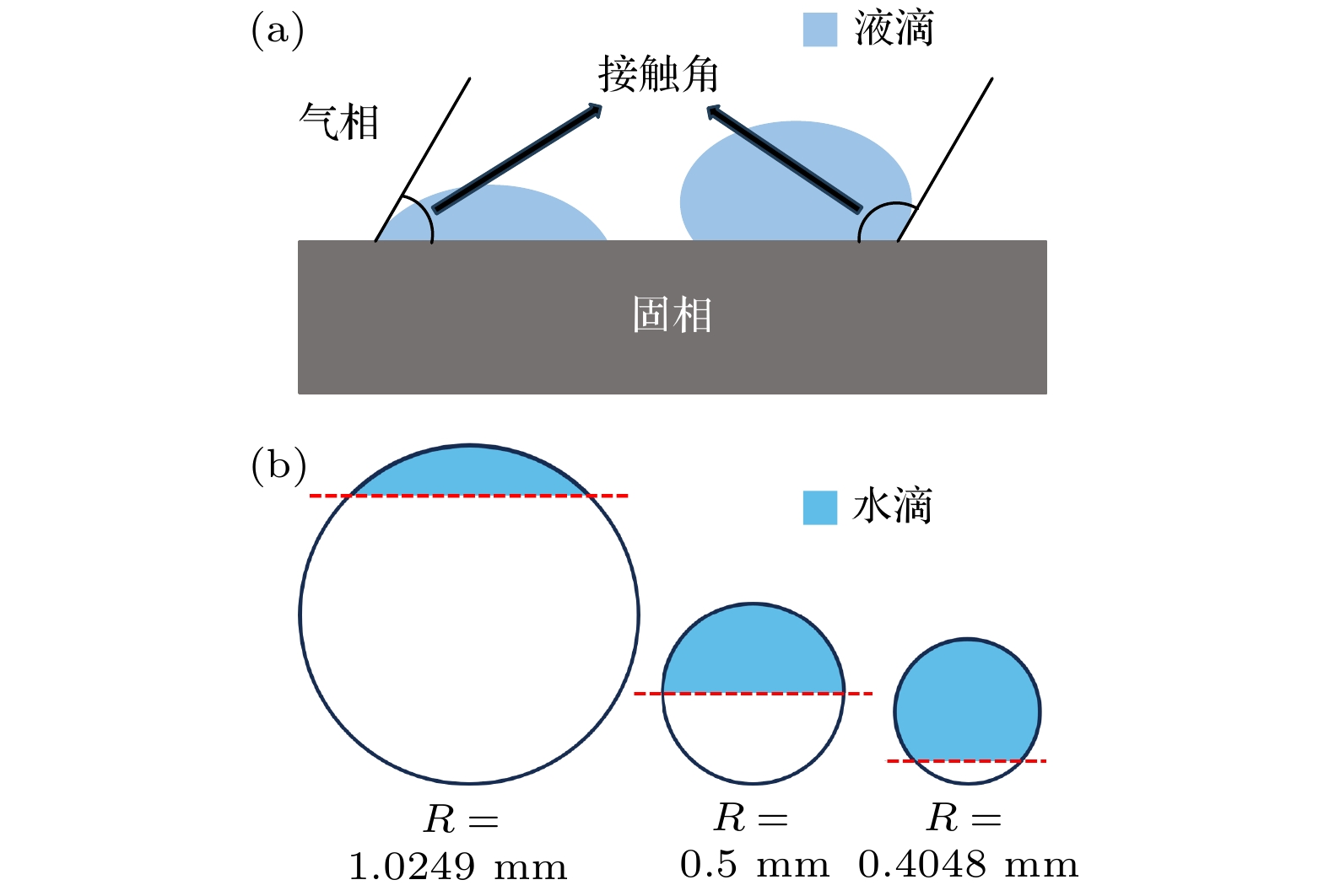
图 3 (a) 液滴接触角θ定义; (b) θ为45°, 90°和135°的水滴的二维几何结构, R为被分割正圆的半径
Fig. 3. (a) The definition of a droplet contact angle θ; (b) two-dimensional geometric structures of water droplets with θ of 45°, 90°, and 135°, R is the radius of the segmented circle.
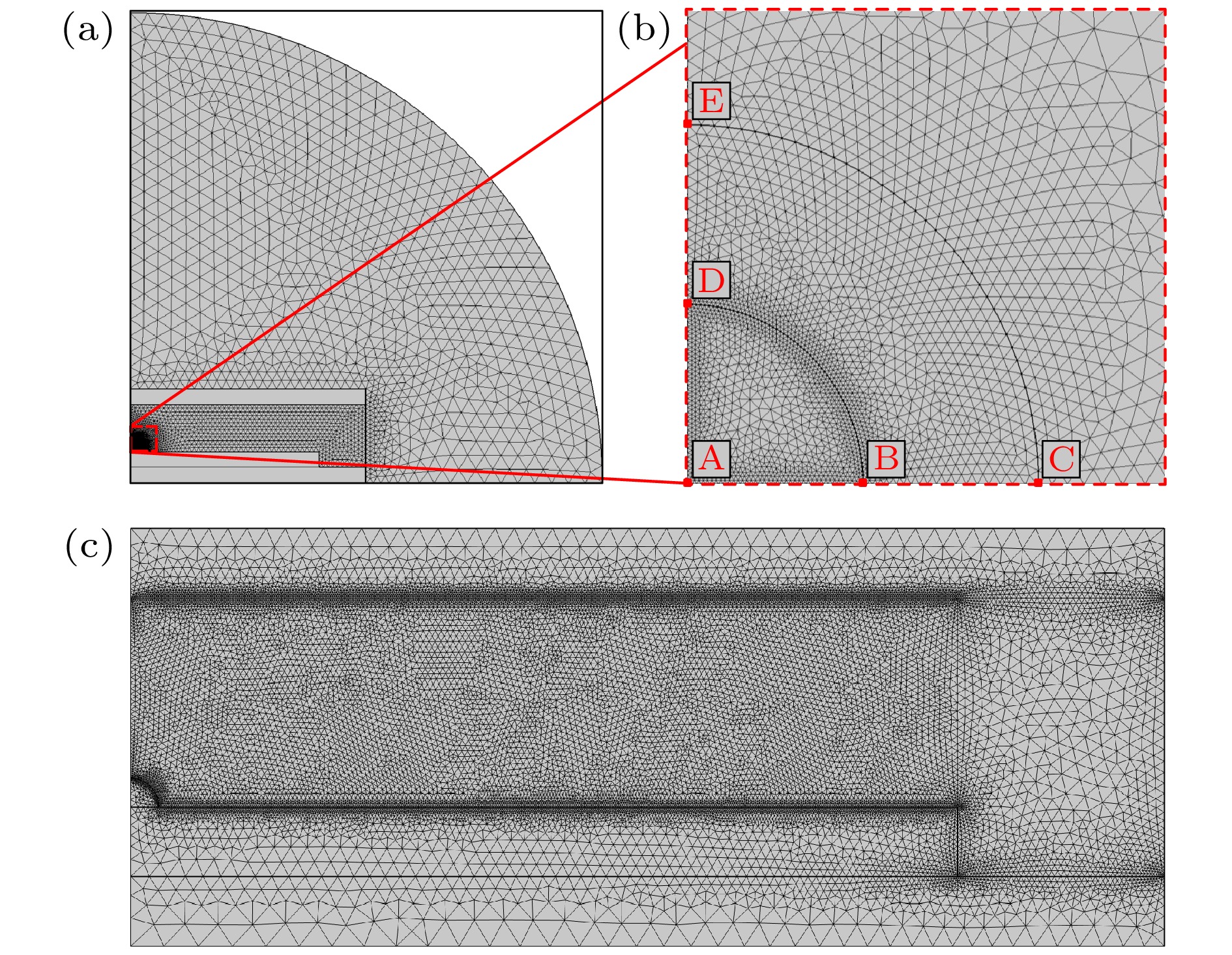
图 4 仿真模型计算域与网格划分 (a) 水滴蒸发流体力学模型与(b) 水滴及周围区域局部放大图; (c) 等离子体流体模型
Fig. 4. The computation domain and grid partitioning of simulation models: (a) The fluid dynamics model of water droplet evaporation and (b) the partial enlarged view of water droplets and surrounding areas; (c) the plasma fluid model.
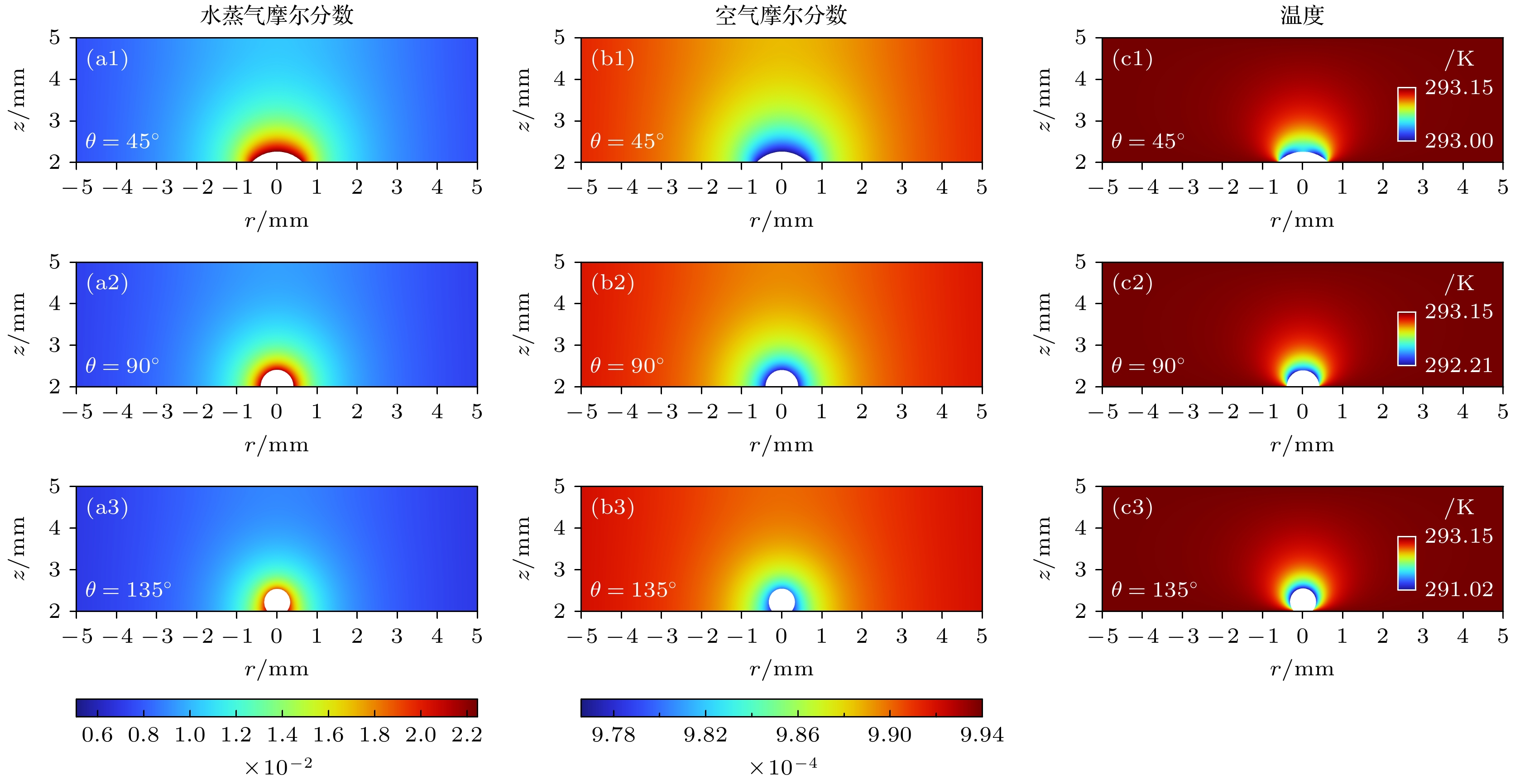
图 5 水滴蒸发150 s后周围区域水蒸气与空气的摩尔分数空间分布以及温度场
Fig. 5. Spatial distributions of mole fractions of water vapor and air in the surrounding area of water droplets after 150 s of evaporation, as well as the temperature field.
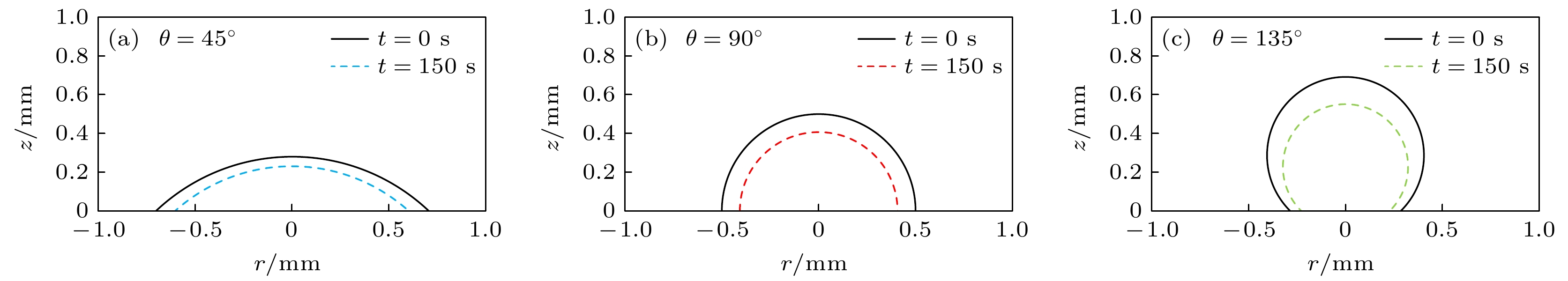
图 6 水滴蒸发150 s前后液面外形曲线
Fig. 6. Shape curves of liquid surfaces of water droplets before and after 150 s of evaporation.
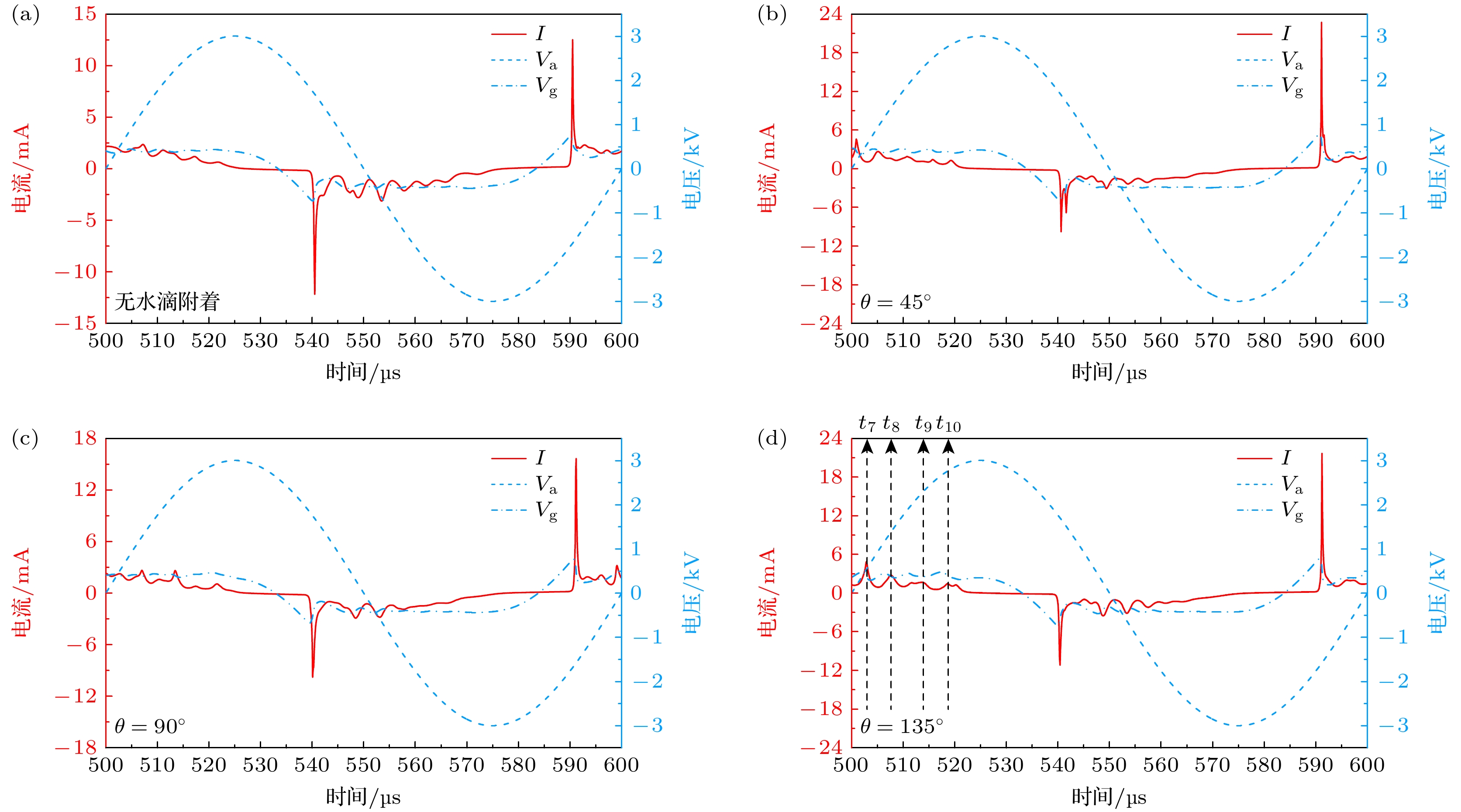
图 7 各情况中DBD的稳态电参数曲线
Fig. 7. Steady-state electrical parameter curves of DBDs in various situations.
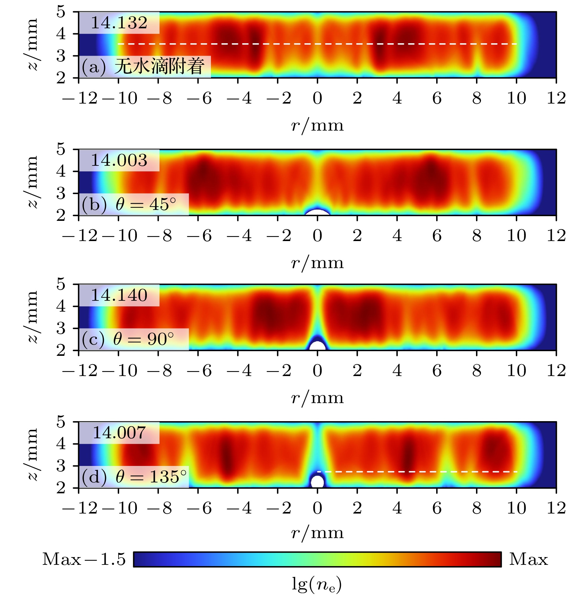
图 8 各情况中DBD的稳态时均对数ne空间分布(ne单位为m–3, 下同), log10(ne)最大值被标注在图中左上角
Fig. 8. Spatial distributions of steady-state time-averaged logarithmic ne of DBDs in various situations (the unit of ne is m–3, the same below), the maximum value of log10(ne) is marked in the upper left corner of figures.
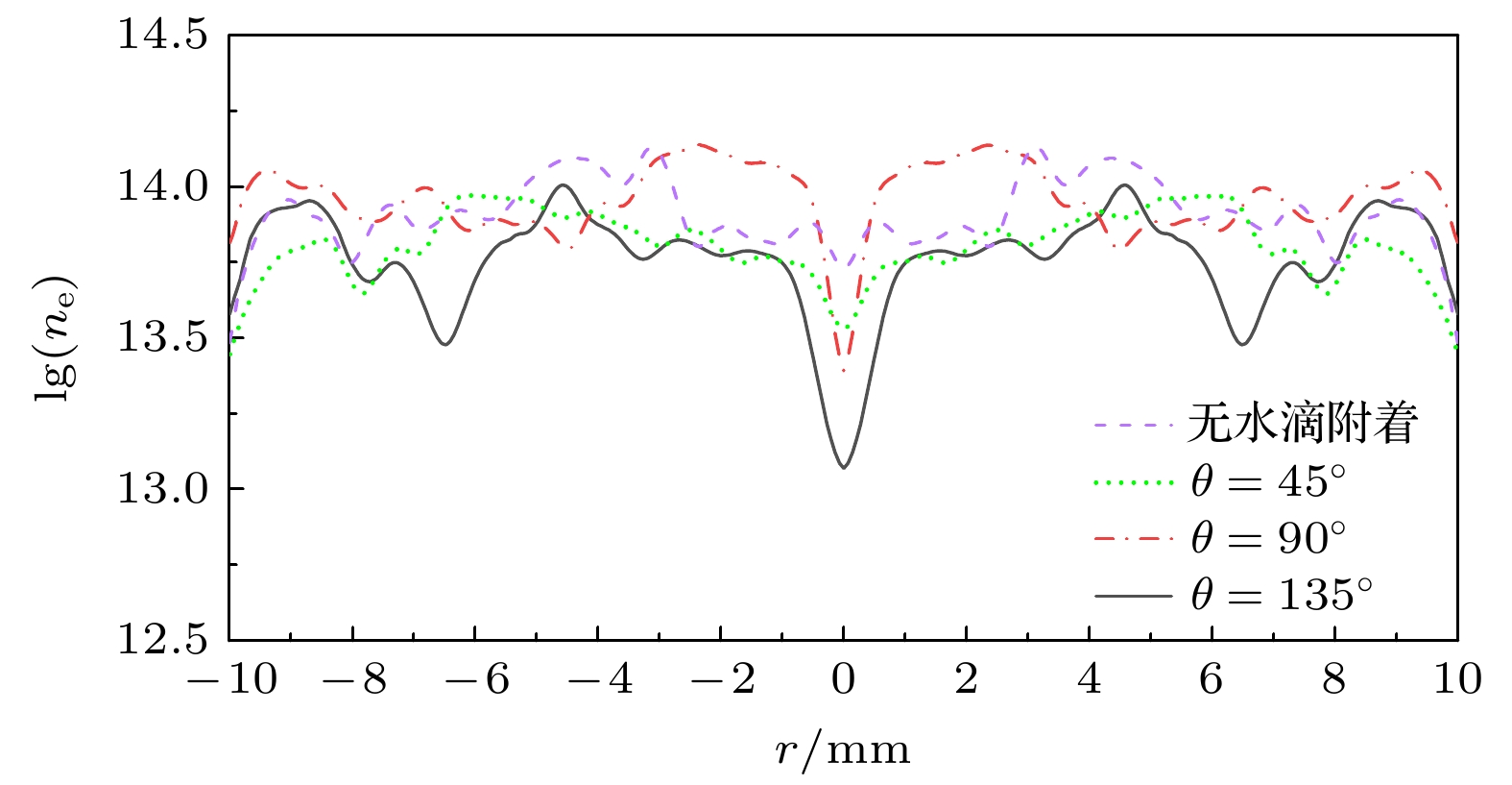
图 9 各情况中沿DBD径向方向的稳态时均对数ne空间分布
Fig. 9. Spatial distributions of steady-state time-averaged logarithmic ne along the radial direction in DBDs in various situations.
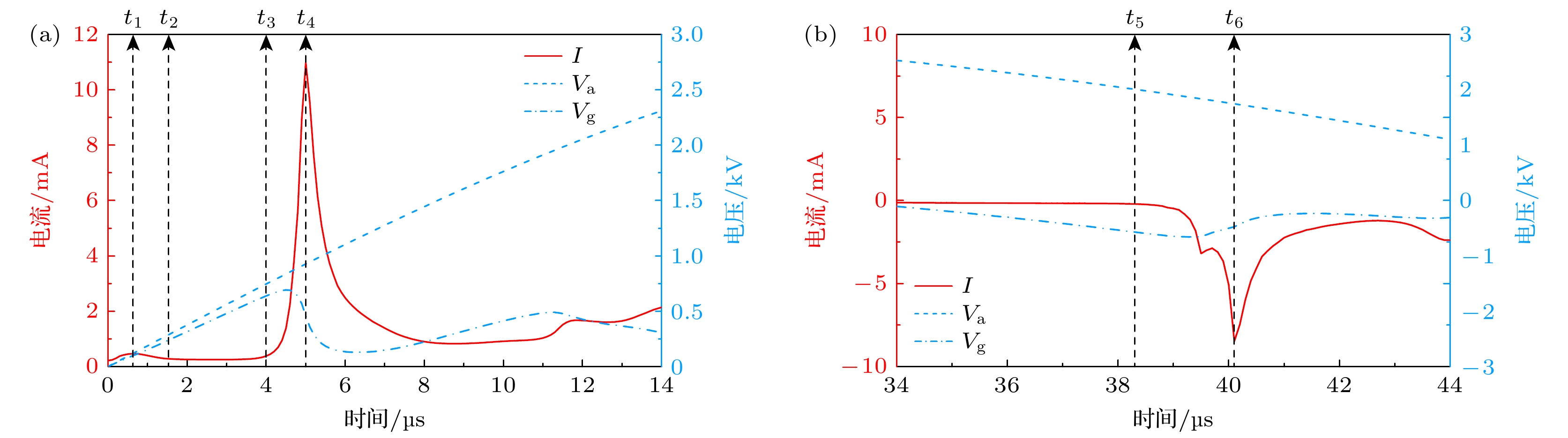
图 10 情况A中DBD的电参数曲线, 第1放电周期主正击穿(a)与主负击穿(b) 时刻附近
Fig. 10. Electrical parameter curves of DBDs in situation A: Near the time of (a) main positive breakdown and (b) main negative breakdown in the first discharge cycle.
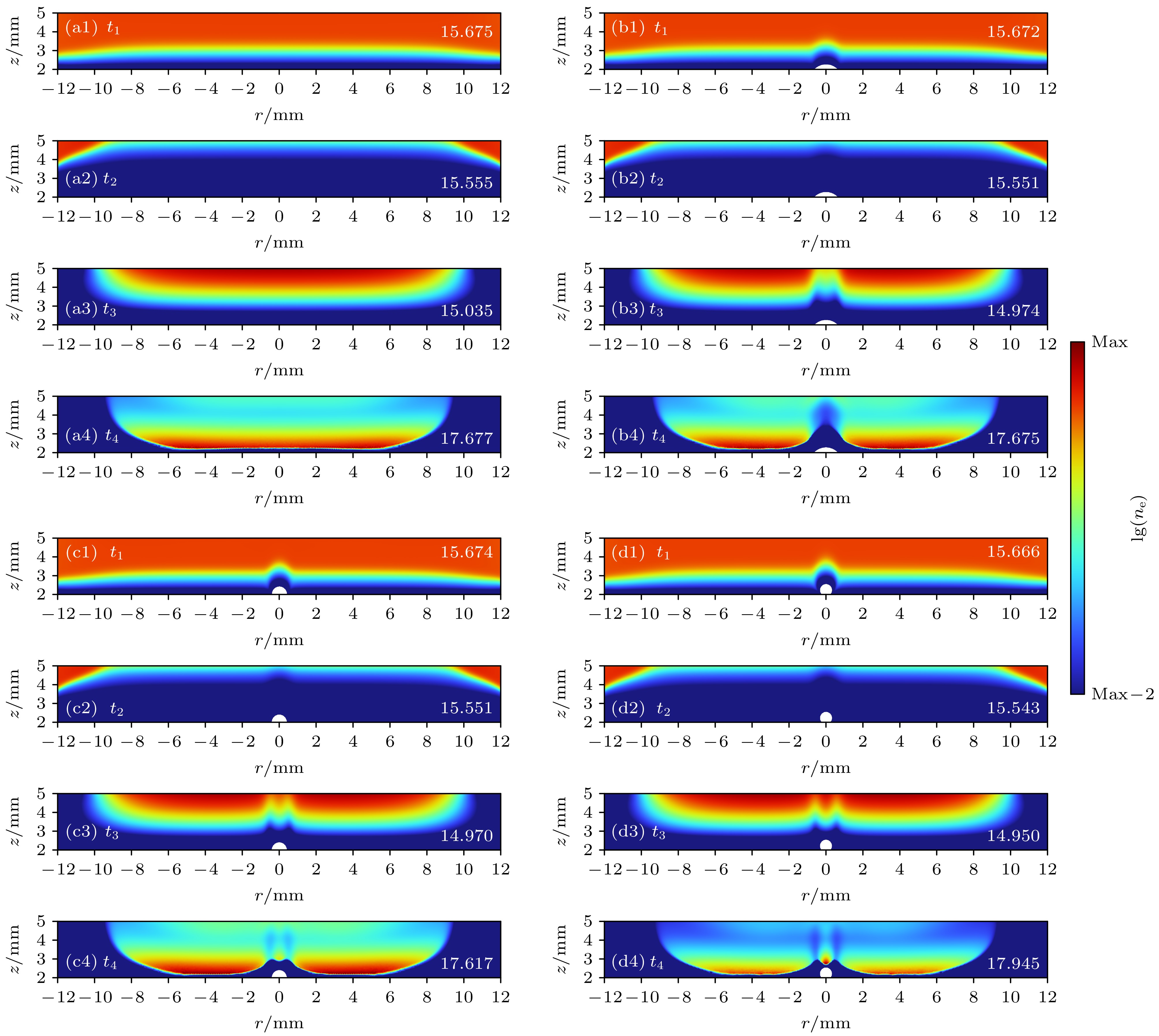
图 11 t1—t4时段DBD的对数ne空间分布, log10(ne)最大值被标注在图中右侧 (a1)—(a4) 情况A; (b1)—(b4) 情况B; (c1)—(c4) 情况C; (d1)—(d4) 情况D
Fig. 11. Spatial distributions of logarithmic ne of DBDs from t1 to t4, the maximum value of log10(ne) is marked in the bottom right corner of figures: (a1)–(a4) Situation A; (b1)–(b4) situation B; (c1)–(c4) situation C; (d1)–(d4) situation D.
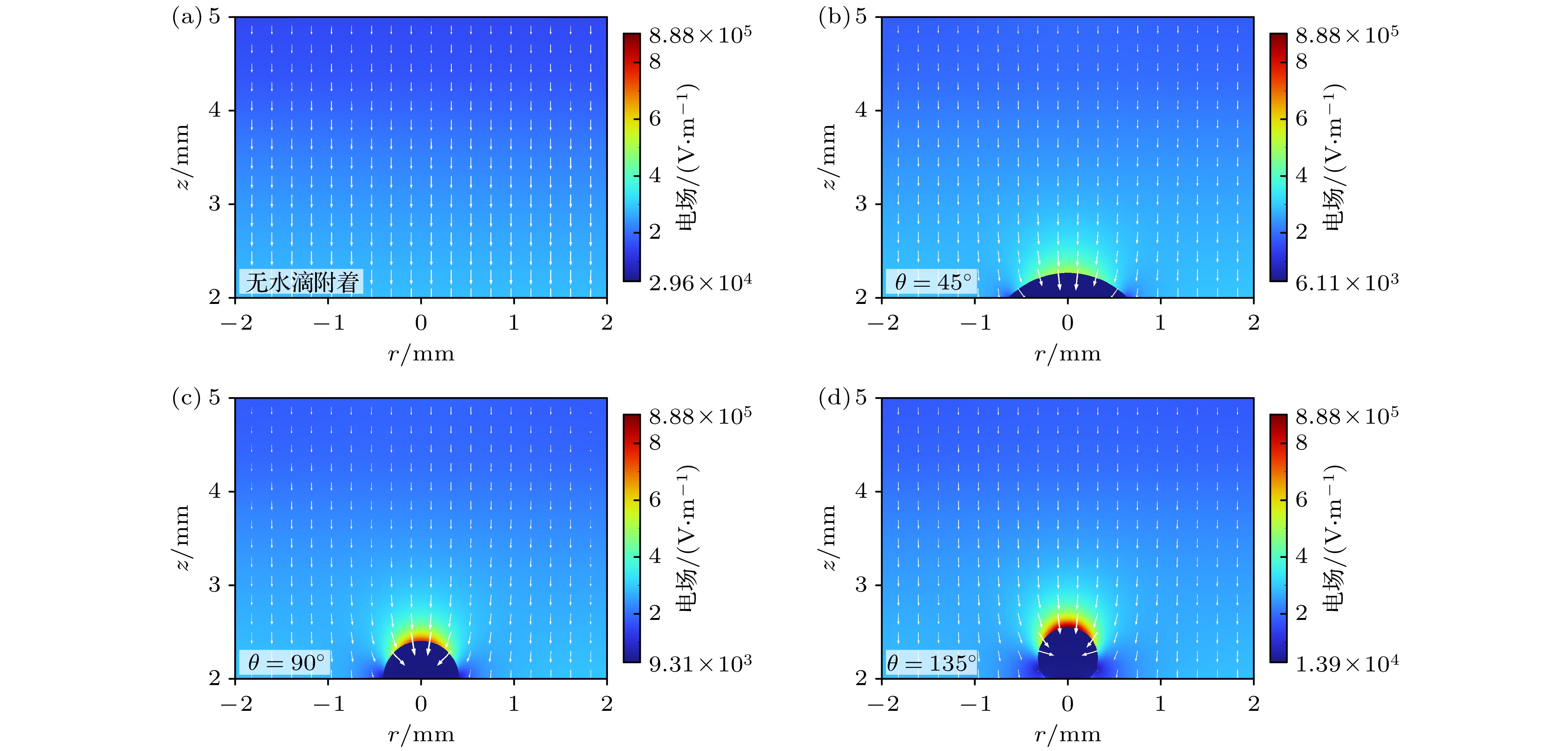
图 12 t3时刻各情况中水滴周围区域电场空间分布
Fig. 12. Spatial distributions of the electric field around water droplets in various situations at t3.
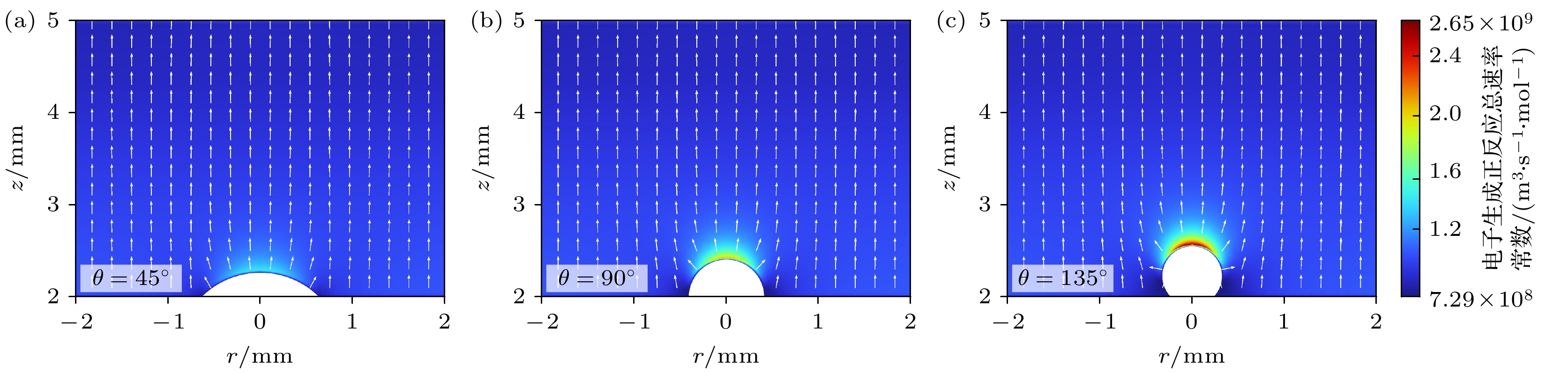
图 13 t3时刻情况B, C, D中水滴周围电子生成总反应速率常数空间分布, 长度归一化的白色箭头表示空间电子通量分布
Fig. 13. Spatial distributions of total reaction rate constants for electron generation around water droplets in situation B, C, and D at t3, the length normalized white arrow represents the spatial electron flux distribution.
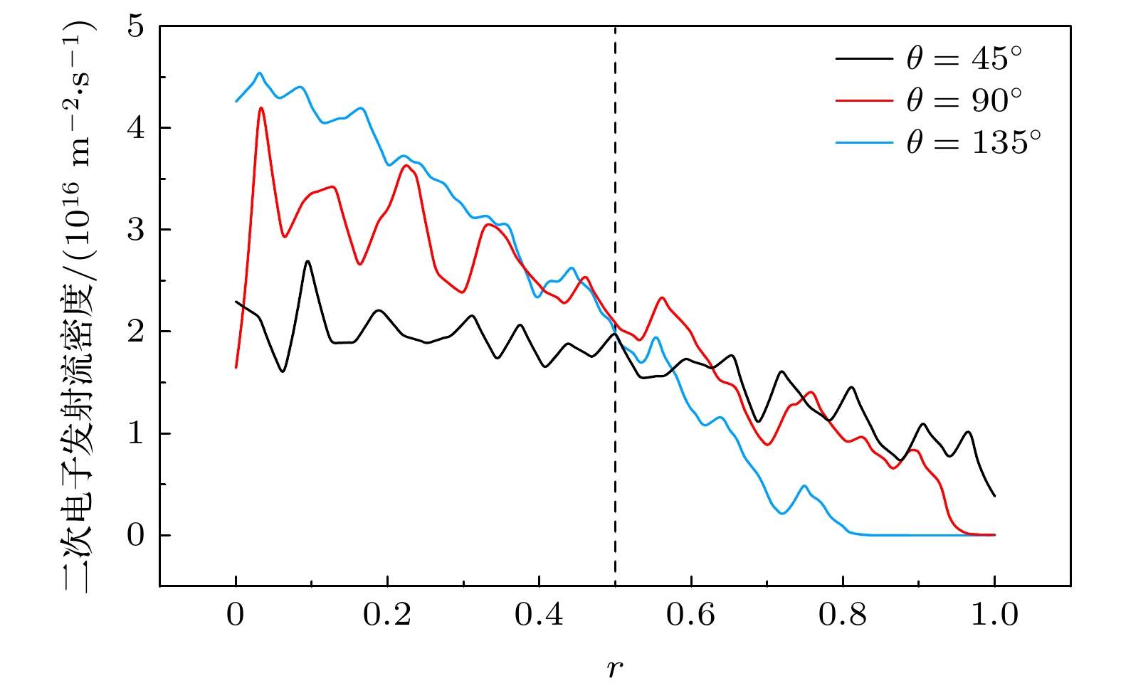
图 14 t3时刻情况B, C, D中水滴表面二次电子发射流密度空间分布
Fig. 14. Spatial distributions of the secondary electron emission flux density on the surface of water droplets in situation B, C, and D at t3.
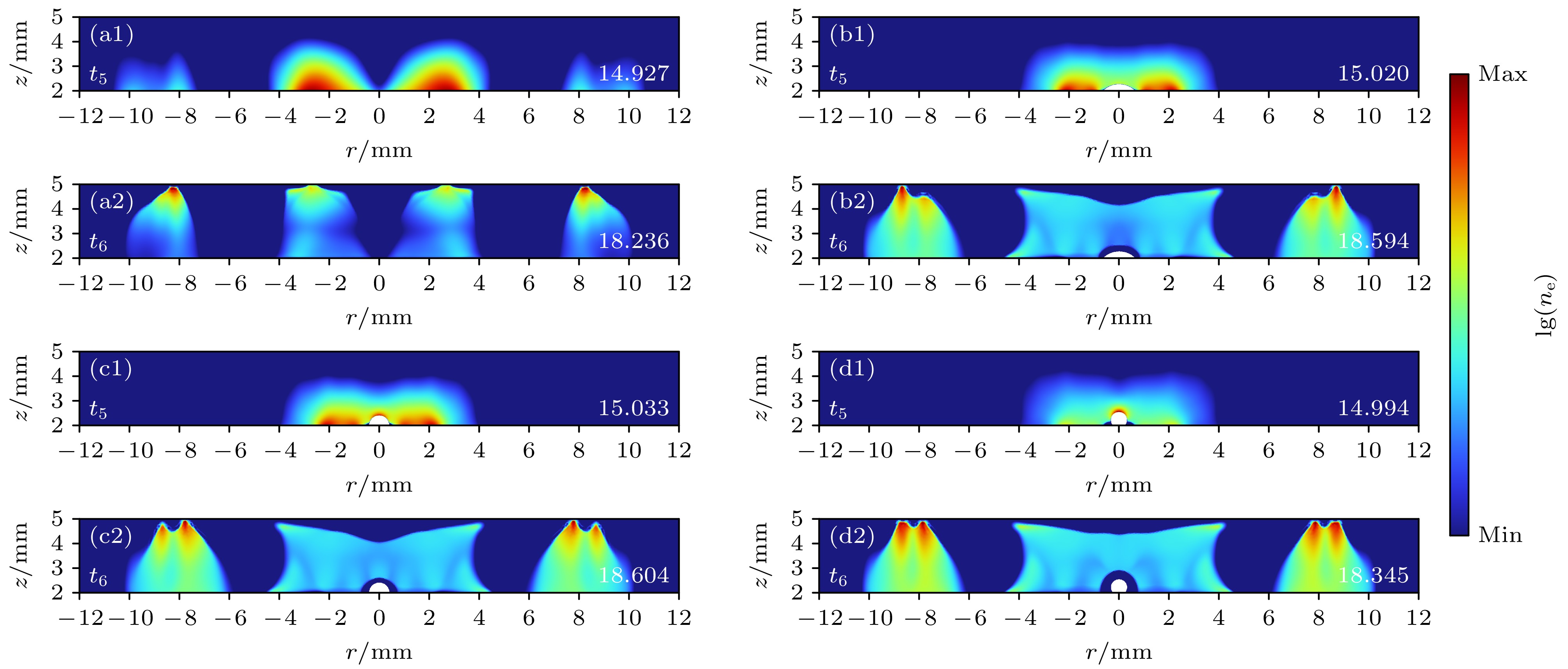
图 15 t5, t6时刻DBD的对数ne空间分布, log10(ne)最大值被标注在图中右下角 (a1), (a2) 情况A; (b1), (b2) 情况B; (c1), (c2) 情况C; (d1), (d2) 情况D
Fig. 15. Spatial distributions of logarithmic ne of DBDs at t5 and t6, the maximum value of log10(ne) is marked in the bottom right corner of figures: (a1), (a2) Situation A; (b1), (b2) situation B; (c1), (c2) situation C; (d1), (d2) situation D.
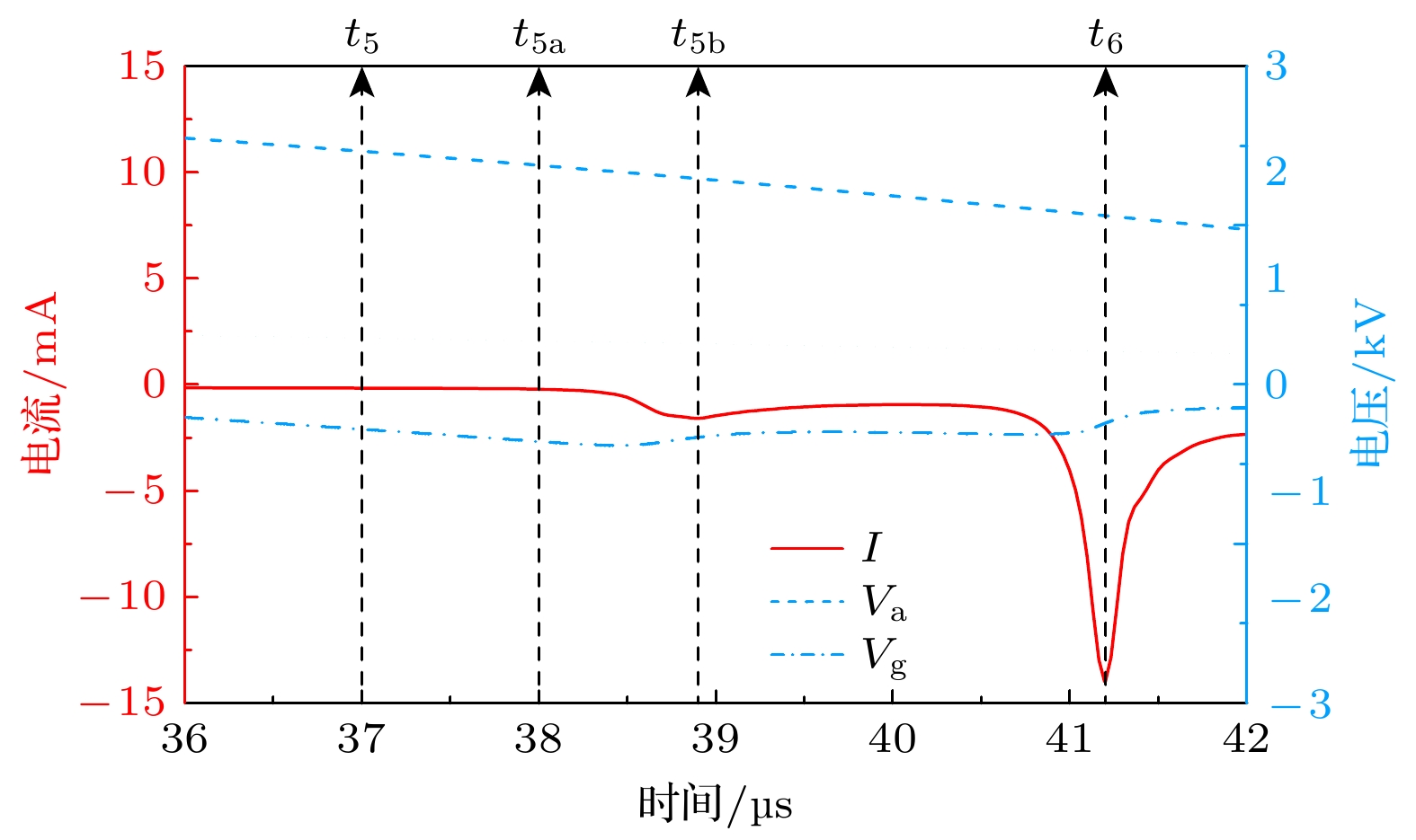
图 16 情况D中DBD的电参数曲线: 第1放电周期主负击穿时刻附近
Fig. 16. Electrical parameter curves of DBDs in situation D: Near the time of main negative breakdown in the first discharge cycle.
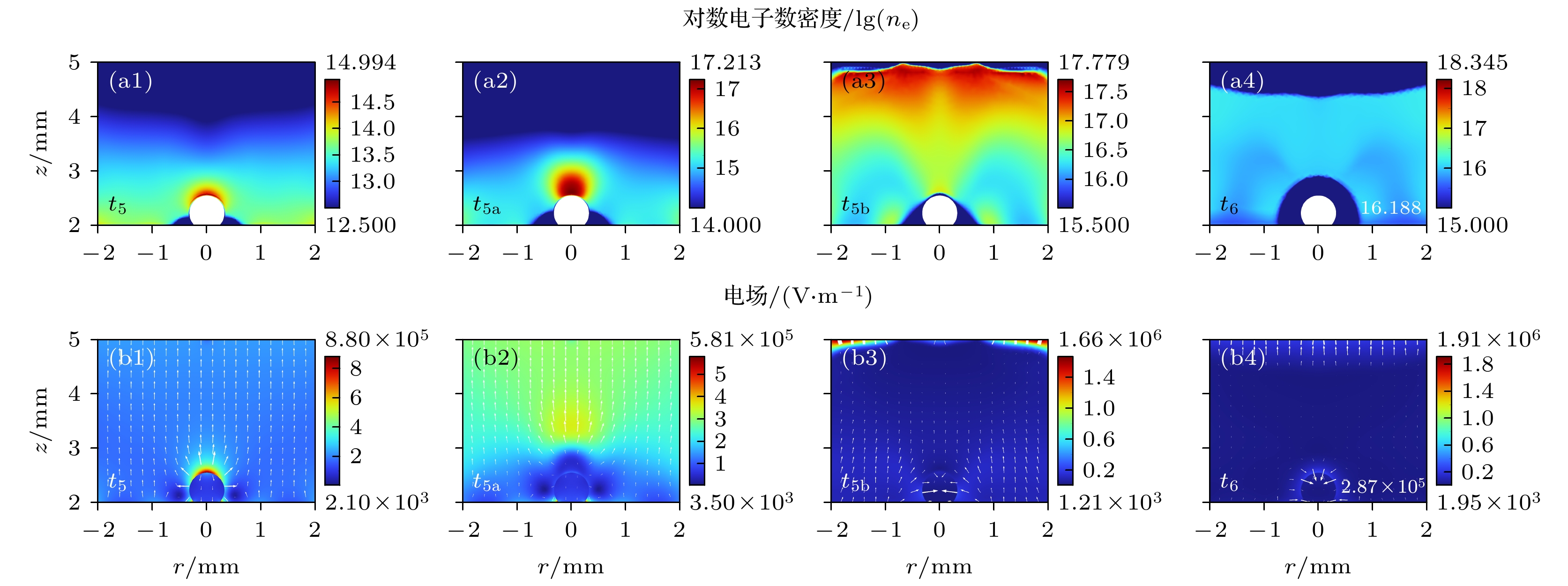
图 17 情况D中t5, t5a, t5b和t6时刻水滴周围区域对数ne与电场空间分布
Fig. 17. Spatial distributions of logarithmic ne and the electric field around water droplets at t5, t5a, t5b and t6 in situation D.
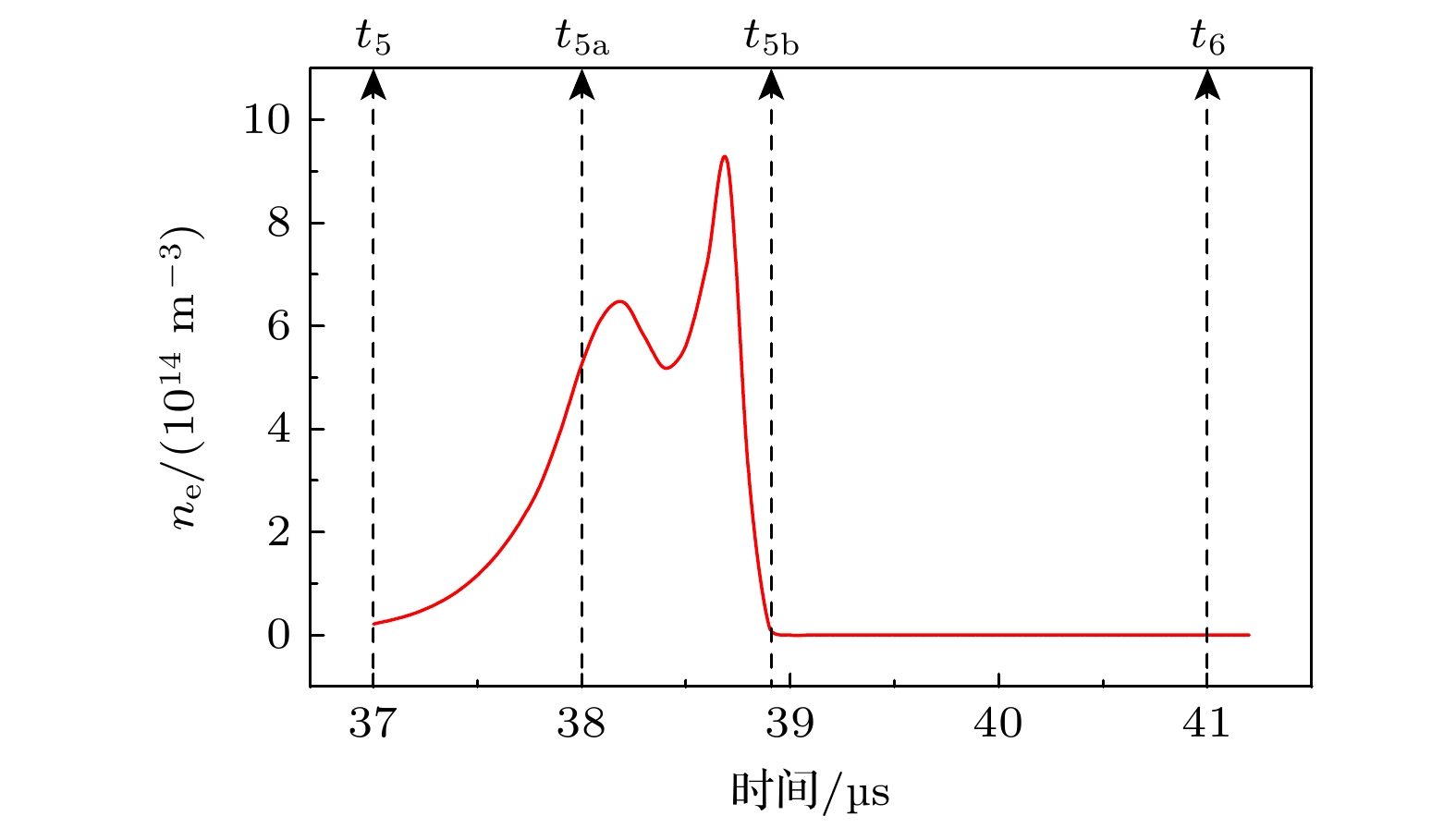
图 18 情况D中t5—t6时段水滴表面平均ne
Fig. 18. Average ne on the surface of the water droplet from t5 to t6 in situation D.
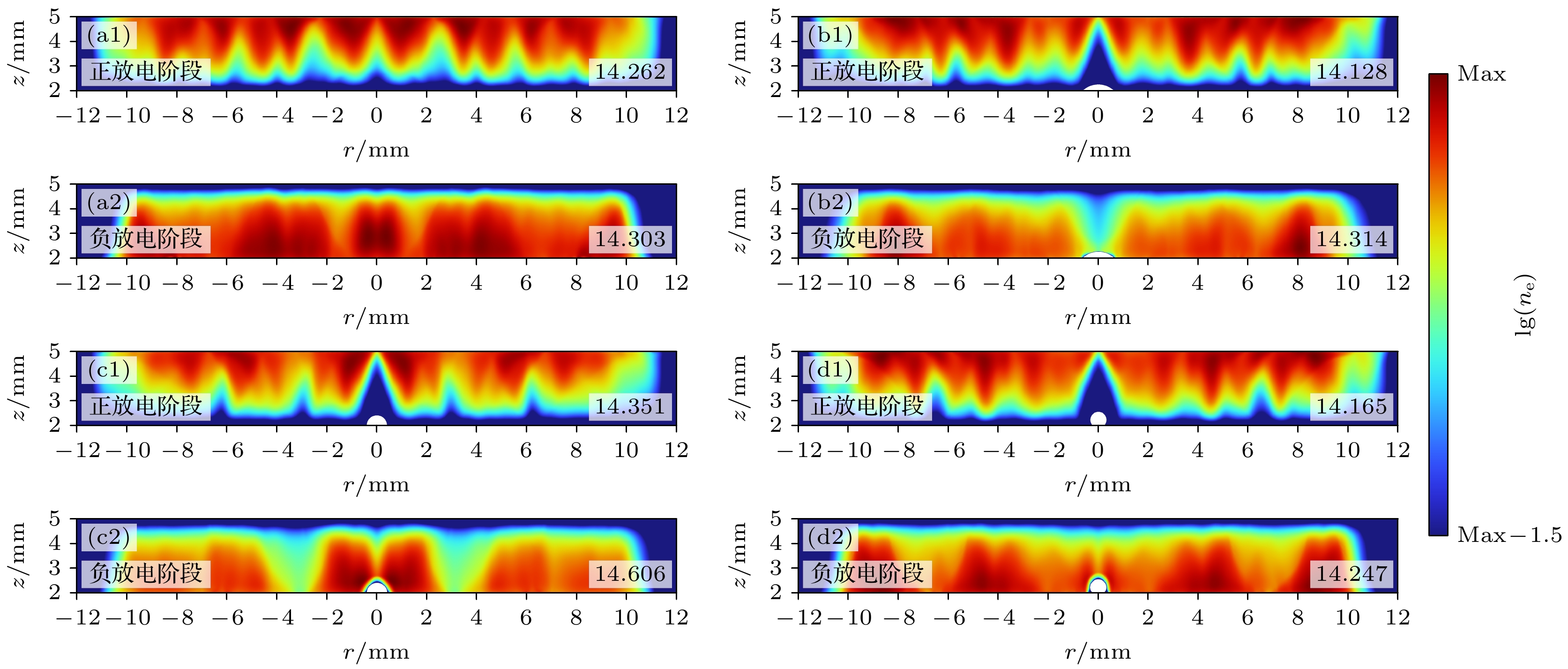
图 19 DBD的稳态正、负放电阶段时均对数ne空间分布, log10(ne)最大值被标注在图中右下角 (a1), (a2) 情况A; (b1), (b2) 情况B; (c1), (c2) 情况C; (d1), (d2) 情况D
Fig. 19. Spatial distributions of time-averaged logarithmic ne during the steady-state positive and negative discharge phases of DBDs, the maximum value of log10(ne) is marked in the bottom right corner of figures: (a1), (a2) Situation A; (b1), (b2) situation B; (c1), (c2) situation C; (d1), (d2) situation D.
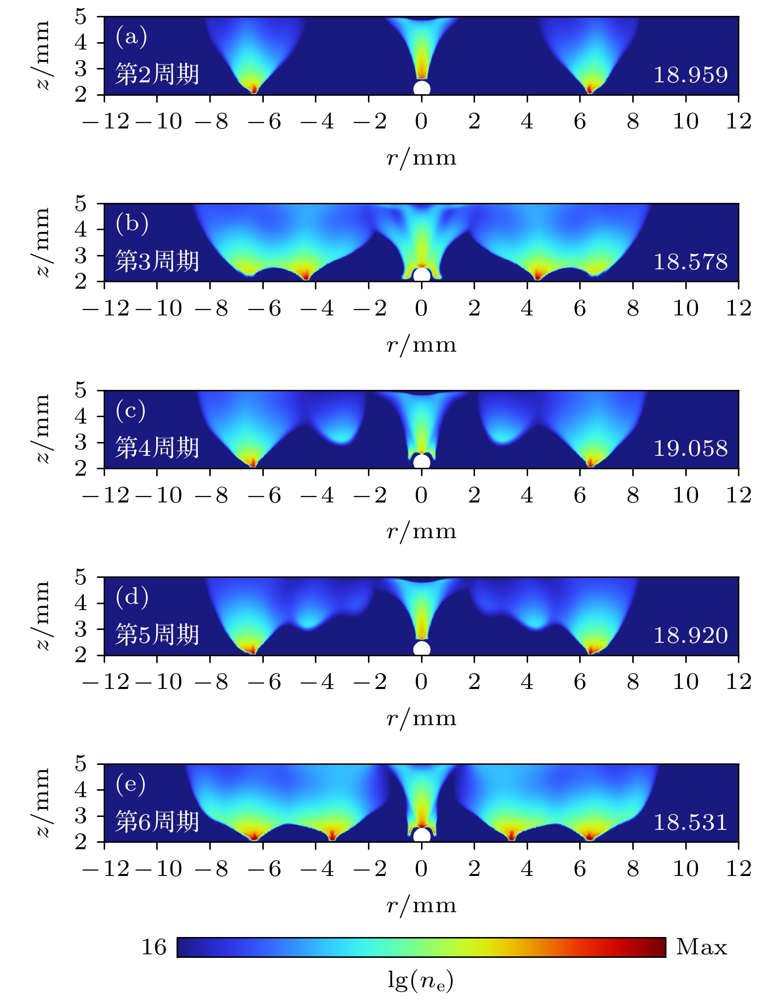
图 20 情况D中第2—6放电周期主正击穿时刻对数ne空间分布, log10(ne)最大值被标注在图中右下角
Fig. 20. Spatial distributions of logarithmic ne at the time of main positive breakdown during the 2nd to 6th discharge cycles in situation D, the maximum value of log10(ne) is marked in the bottom right corner of figures.
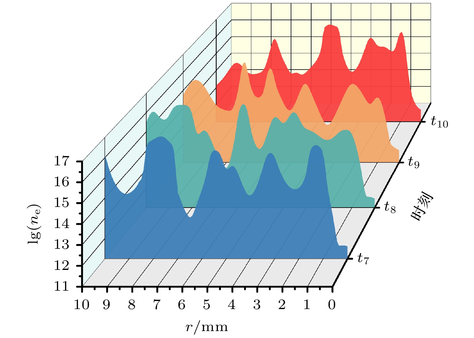
图 21 情况D中t7—t10时段径向对数ne空间分布
Fig. 21. Radial spatial distributions of logarithmic ne from t7 to t10 in situation D.
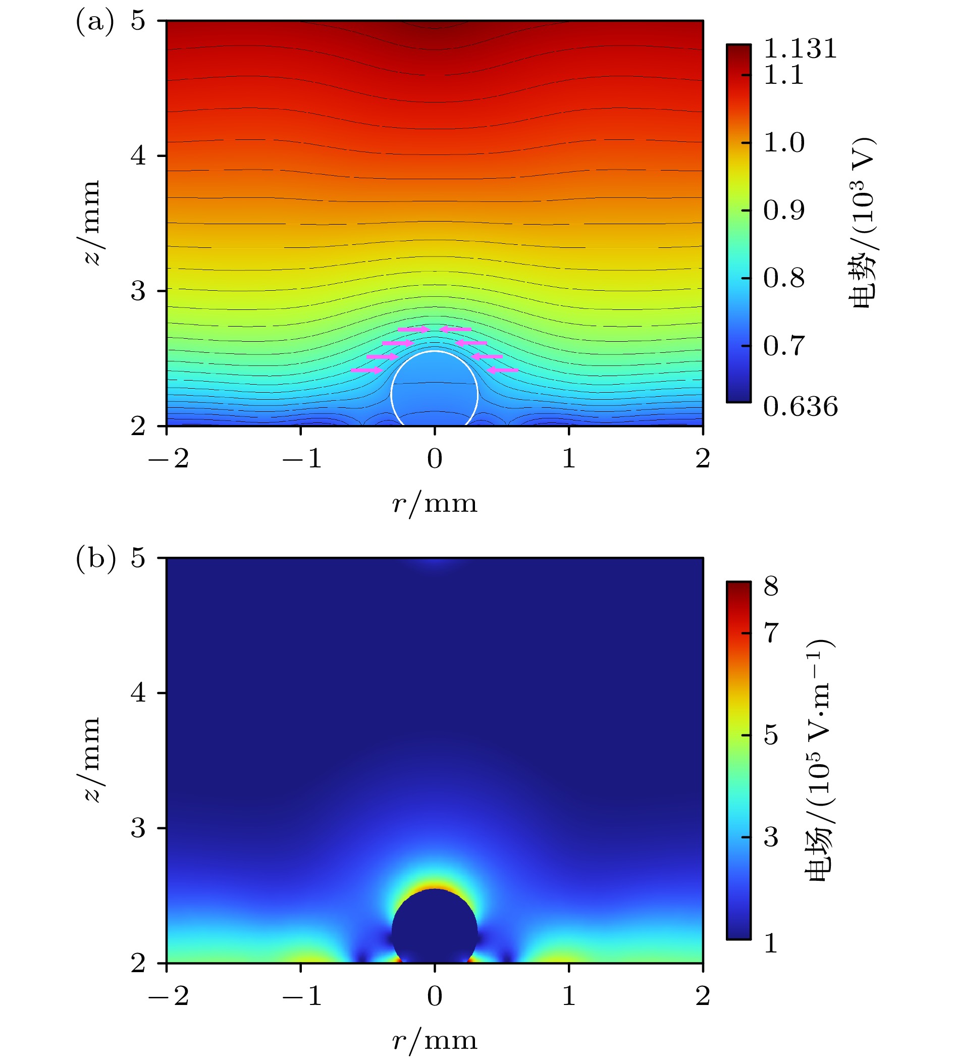
图 22 情况D中t7—t10时段时均电势与时均场强空间分布
Fig. 22. Spatial distributions of time-averaged potential and time-averaged electric field strength from t7 to t10 in situation D.
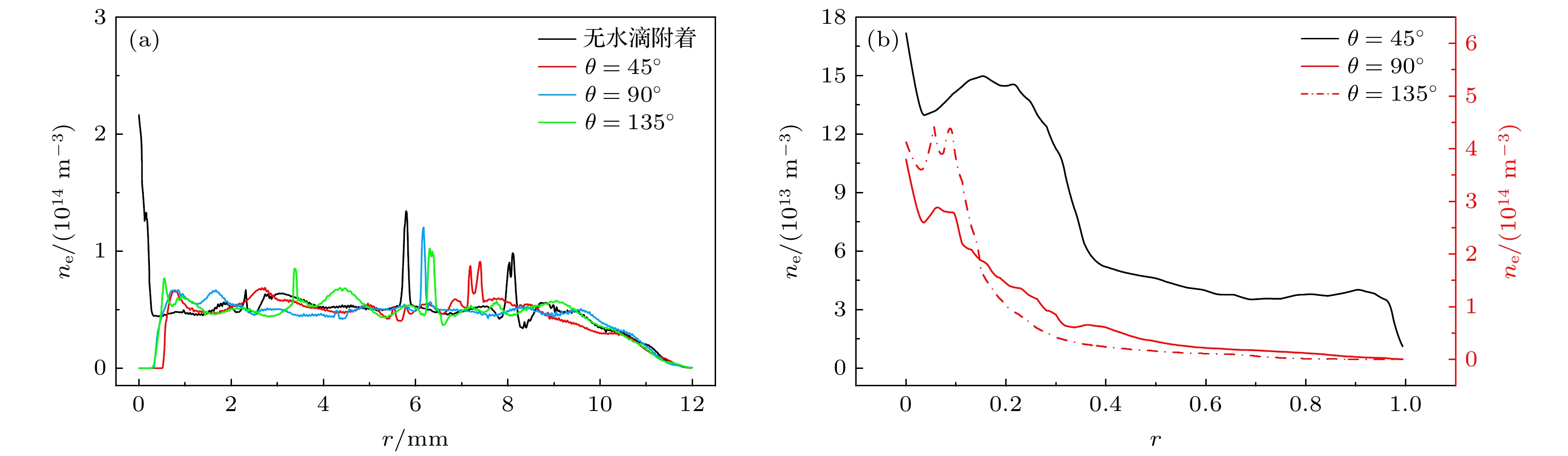
图 23 各情况中稳态时均ne空间分布 (a) 待处理物表面; (b) 水滴表面
Fig. 23. Spatial distributions of steady-state time-averaged ne on the surface of (a) specimens to be treated and (b) water droplets in various situations.
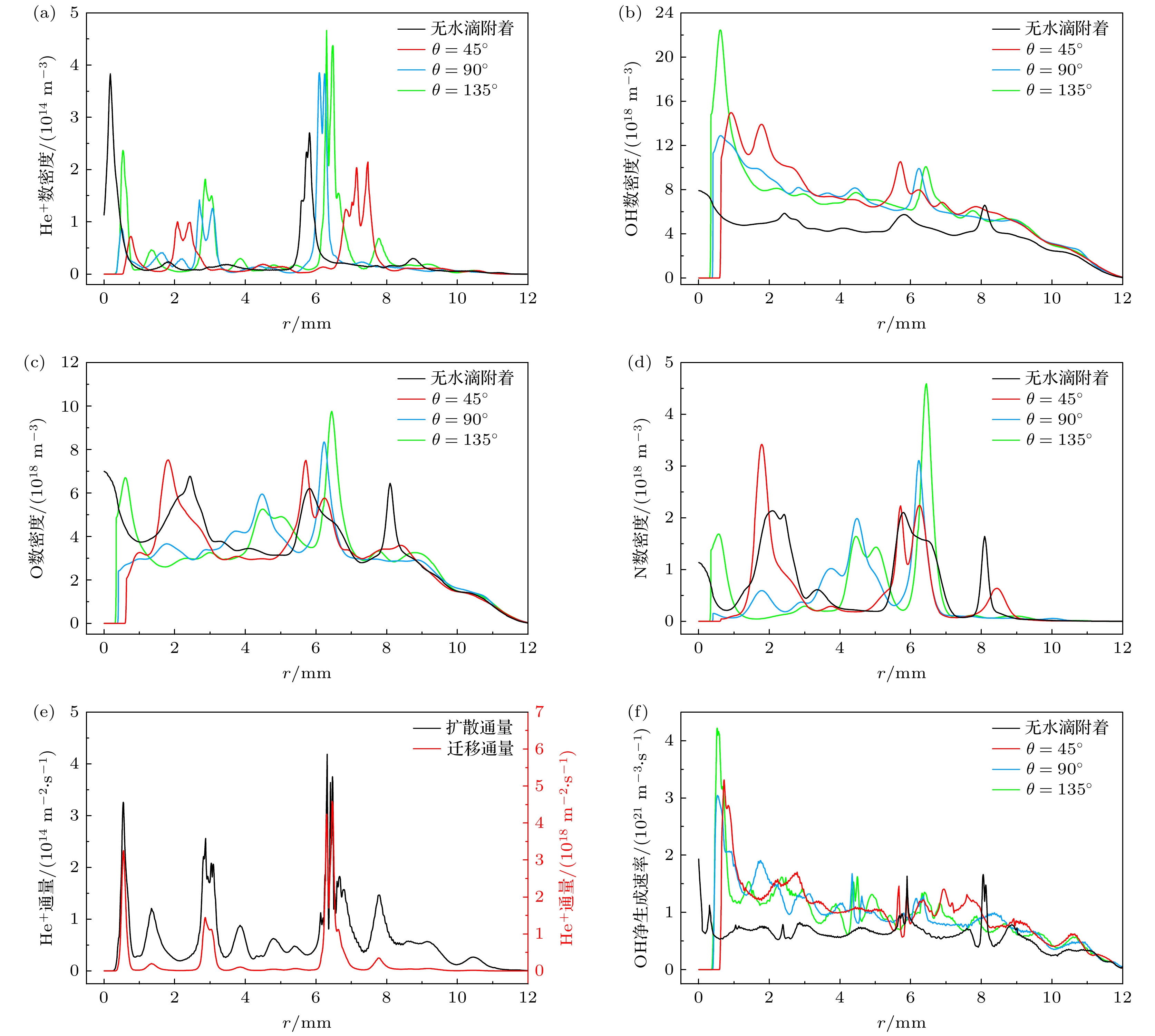
图 24 待处理物表面稳态时均数据的空间分布 (a)—(d) 各情况中活性粒子的数密度; (e) 情况D中He+的通量; (f) 各情况中OH的净生成速率
Fig. 24. Spatial distributions of steady-state time-averaged data on the surface of specimens to be treated: (a)–(d) Active particle number density in various situations; (e) He+ flux in situation D; (f) net generation rate of OH in various situations.
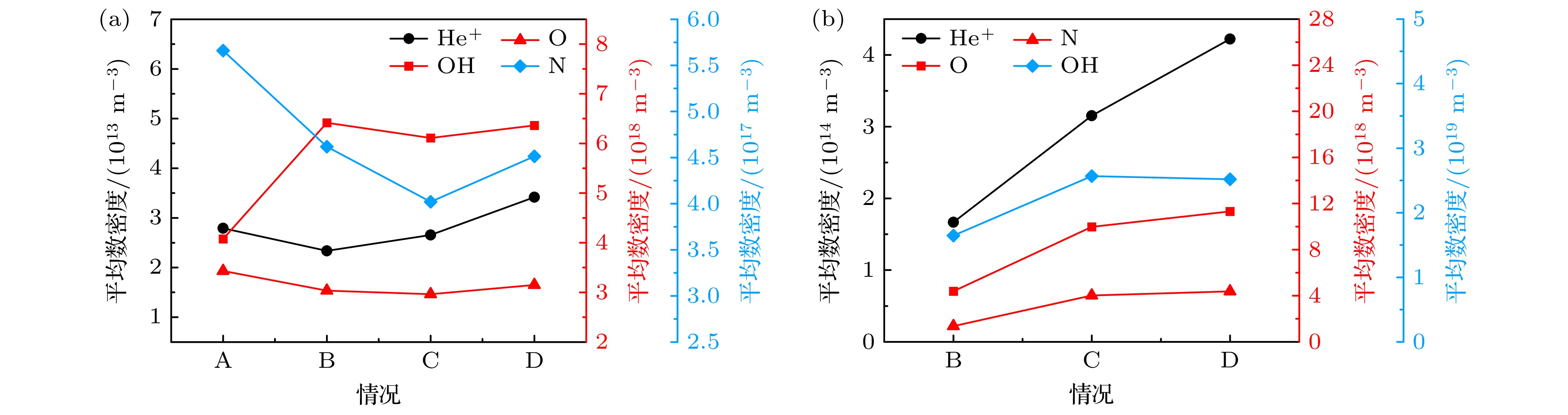
图 25 各情况中活性粒子稳态时均数密度的平均值 (a) 待处理物表面; (b) 水滴表面
Fig. 25. Average values of steady-state time-averaged active particle number density on the surface of (a) specimens to be treated and (b) water droplets in various situations.
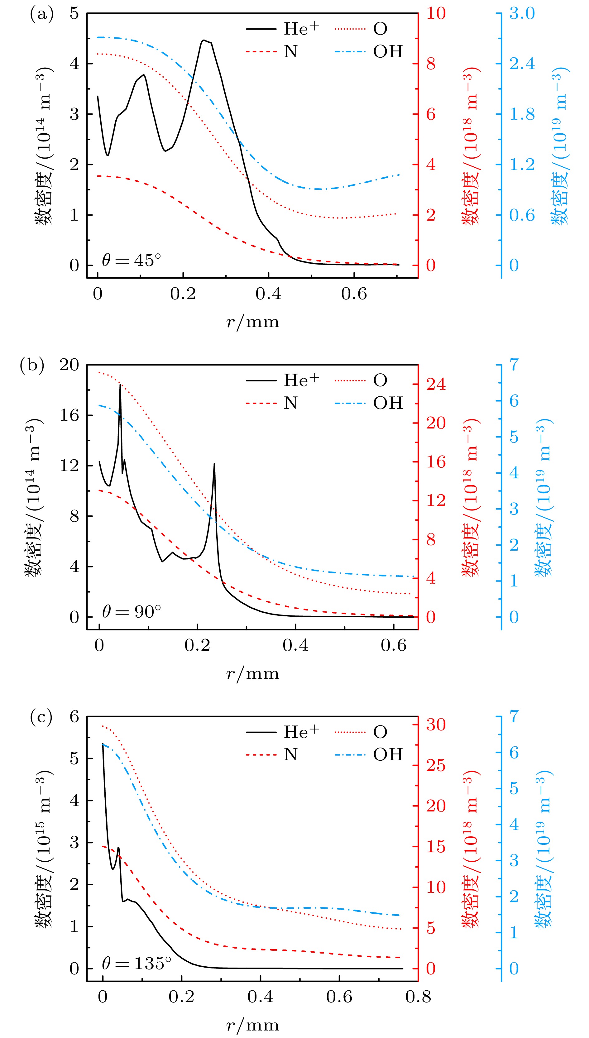
图 26 θ不同的水滴表面活性粒子稳态时均数密度空间分布
Fig. 26. Spatial distributions of steady-state time-averaged active particle number density on the surface of water droplets with different θ.
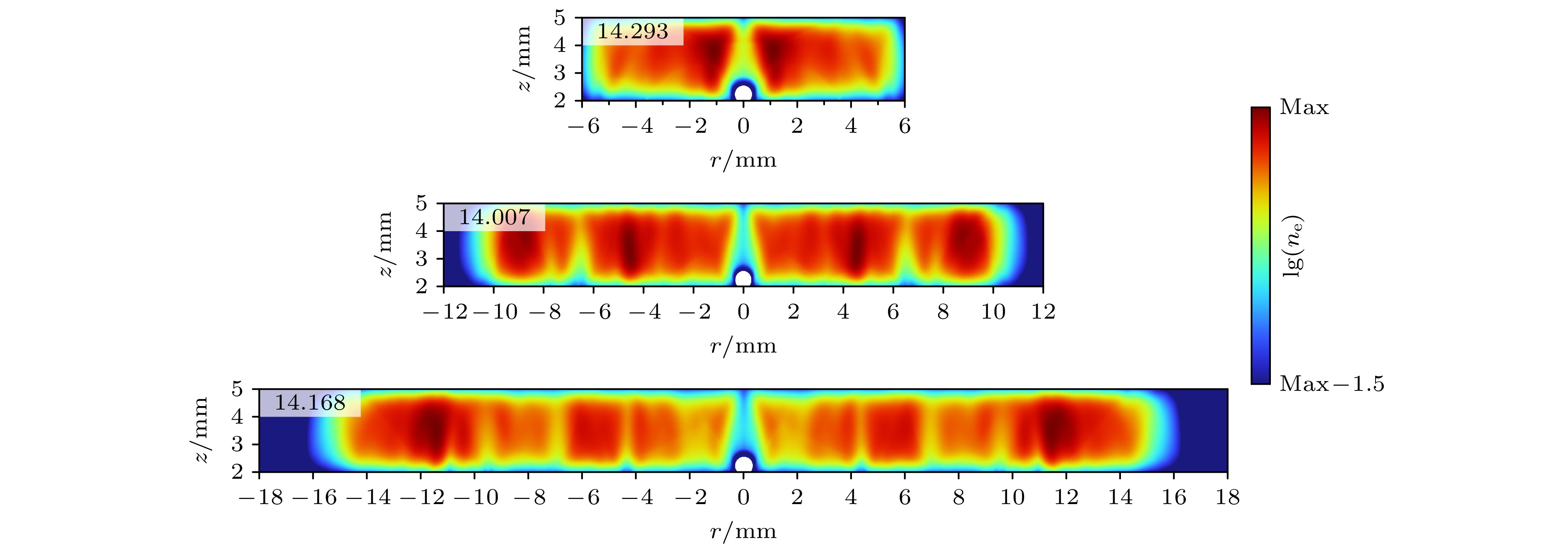
图 A1 在模型径向尺寸缩小比例不同的情况下, 情况D中DBD的稳态放电结构, log10(ne)最大值被标注在图中左上角
Fig. A1. The steady-state discharge structure of DBDs in situation D under different radial size reduction ratios of the model, the maximum value of log10(ne) is marked in the upper left corner of figures.
表 A1 等离子体化学反应体系
Table A1. Chemical reaction system of plasma.
序号 反应式 速率系数 焓变/eV 参考文献 1 $ {\text{e}}+{\text{He}} \to {\text{e} + \text{He}} $ f(c, ε) — [43] 2 $ {\text{e}}+{\text{He}} \to {\text{e} + \text{H}}{{\text{e}}^ * } $ f(c, ε) 19.82 [43] 3 $ {\text{e}}+{{\text{He}}^ * } \to {\text{e} + \text{He}} $ 2.9×10⁻¹⁵ –19.82 [43] 4 $ {\text{e}}+{\text{He}} \to 2{\text{e} + \text{H}}{{\text{e}}^ + } $ f(c, ε) 24.58 [43] 5 $ {\text{e}}+{{\text{He}}^ * } \to 2{\text{e} + \text{H}}{{\text{e}}^ + } $ $4.661\times 10^{-16}\times T_{\rm e}^{0.6} \times \exp(-4.78/T_{\rm e}) $ 4.78 [43] 6 $ {\text{e}}+{\text{He}}_2^ * \to 2{\text{e} + \text{He}}_2^ + $ $1.268 \times 10^{-18}\times T_{\rm e}^{0.71} \times\exp (-3.4/T_{\rm e}) $ 3.4 [43] 7 $ {\text{e}}+{\text{He}}_2^ + \to {{\text{He}}^ * }+{\text{He}} $ $5.386\times 10^{-13}\times T_{\rm e}^{-0.5} $ — [10] 8 $ {\text{e}}+{{\text{He}}^ + } \to {\mathrm{He}}^ * $ $6.76\times 10^{-19}\times T_{\rm e}^{-0.5} $ — [10] 9 $ 2{\text{e}} + {{\text{He}}^ + } \to {\text{e}}+{{\text{He}}^ * } $ $6.186\times 10^{-39}\times T_{\rm e}^{-4.4} $ — [10] 10 $ {\text{e} + \text{He}}+{{\text{He}}^ + } \to \text{He}+{{\text{He}}^ * } $ $6.66\times 10^{-42}\times T_{\rm e}^{-2} $ — [10] 11 $ 2 {\text{e} + \text{He}}_2^ + \to \text{He}_2^ * + {\text{e}} $ 1.2×10⁻³³ — [10] 12 $ {\text{e} + \text{He} + \text{He}}_2^ + \to \text{He}_2^ * + {\text{He}} $ 1.5×10–39 — [10] 13 $ {\text{e} + \text{He} + \text{He}}_2^ + \to {\mathrm{He}}^ * + 2 {\text{He}} $ 3.5×10–39 — [10] 14 $ 2 {\text{e} + \text{He}}_2^ + \to \text{He}^ * +{\text{He} + \text{e}} $ 2.8×10⁻³² — [10] 15 $ {\text{e}}+{{\text{N}}_2} \to {\text{e}}+{{\text{N}}_2} $ f(c, ε) — [43] 16 $ {\text{e}}+{{\text{N}}_2} \to {\text{e}}+{{\text{N}}_2} $ (v = 1) f(c, ε) 0.29 [55] 17 $ {\text{e}}+{{\text{N}}_2} \to {\text{e}}+{{\text{N}}_2} $ (v = 2) f(c, ε) 0.59 [55] 18 $ {\text{e}}+{{\text{N}}_2} \to {\text{e}}+{{\text{N}}_2} $ (v = 3) f(c, ε) 0.856 [10] 19 $ {\text{e}}+{{\text{N}}_2} \to {\text{e}}+{{\text{N}}_2} $ (v = 4) f(c, ε) 1.134 [10] 20 $ {\text{e}}+{{\text{N}}_2} \to {\text{e}}+{{\text{N}}_2} $ (v = 5) f(c, ε) 1.4088 [43] 21 $ {\text{e}}+{{\text{N}}_2} \to 2{\text{e} + \text{N}}_2^ + $ f(c, ε) 15.6 [55] 22 $ {\text{e} + \text{N}}_4^ + \to 2\text{N}_2 $ $3.18\times 10^{-13}\times T_{\rm e}^{-0.5} $ — [10] 23 $ {\text{e} + \text{N}}_2^ + \to 2 {\mathrm{N}} $ $4.8 \times 10^{-13} \times T_{\rm e}^{-0.5} $ — [10] 24 $ {\text{e} + \text{N}}_2^ + \to \text{N}_2 $ $7.72\times 10^{-14} \times T_{\rm e}^{-0.5} $ — [10] 25 $ {\text{e}}+{{\text{O}}_2} \to {\text{e}}+{{\text{O}}_2} $ f(c, ε) — [55] 26 $ {\text{e}}+{{\text{O}}_2} \to {\mathrm{O}}+{{\text{O}}^ - } $ f(c, ε) — [55] 27 $ {\text{e}}+{{\text{O}}_2} \to {\text{e}}+{{\text{O}}_2} $ (v = 3) f(c, ε) 0.57 [55] 28 $ {\text{e}}+{{\text{O}}_2} \to {\text{e}}+{{\text{O}}_2} $ (v = 4) f(c, ε) 0.75 [55] 29 $ {\text{e}}+{{\text{O}}_2} \to {\text{e}}+{{\text{O}}_2} $ (a1) f(c, ε) 0.977 [55] 30 $ {\text{e}}+{{\text{O}}_2} \to {\text{e}}+{{\text{O}}_2} $ f(c, ε) –0.977 [10] 31 $ {\text{e}}+{{\text{O}}_2} \to {\text{e}}+{{\text{O}}_2} $ (b1) f(c, ε) 1.627 [55] 32 $ {\text{e}}+{{\text{O}}_2} \to {\text{e}}+{{\text{O}}_2} $ f(c, ε) –1.627 [10] 33 $ {\text{e}}+{{\text{O}}_2} \to {\text{e}}+{{\text{O}}_2} $ (EXC) f(c, ε) 4.5 [55] 34 $ {\text{e}}+{{\text{O}}_2} \to {\text{O}}_2^ - $ f(c, ε) — [43] 35 $ {\text{e}}+{{\text{O}}_2} \to {\text{e + O + O}} $ f(c, ε) 5.58 [10] 36 $ {\text{e}}+{{\text{O}}_2} \to {\text{e + O + O}} $ (1D) f(c, ε) 8.4 [10] 37 $ {\text{e}}+{{\text{O}}_2} \to 2{\text{e} + \text{O}}_2^ + $ f(c, ε) 12.06 [55] 38 $ {\text{e}} + 2{{\text{O}}_2} \to \text{O}_2+{\text{O}}_2^ - $ $5.17\times 10^{-43} \times T_{\rm e}^{-1} $ –0.43 [43] 39 $ {\text{e} + \text{O}}_2^ + \to 2{\text{O}} $ $6\times 10^{-11} \times T_{\rm e}^{-1} $ –6.91 [43] 40 $ {\text{e} + \text{O}}_2^ + \to \text{O}_2 $ 4×10–18 — [43] 41 $ {\text{e} + \text{O}}_4^ + \to 2\text{O}_2 $ $2.25\times 10^{-13}\times T_{\rm e}^{-0.5} $ — [10] 42 $ {\text{e}}+{{\text{H}}_2}{\text{O}} \to {\text{e}}+{{\text{H}}_2}{\text{O}} $ f(c, ε) — [10] 43 $ {\text{e}}+{{\text{H}}_2}{\text{O}} \to {\text{e + e + }}{{\text{H}}_2}{{\text{O}}^ + } $ f(c, ε) 13.76 [10] 44 $ {\text{e}}+{{\text{H}}_2}{\text{O}} \to {\text{e + H + OH}} $ f(c, ε) 7 [10] 45 $ {\text{e + H + OH}} \to {\text{e}}+{{\text{H}}_2}{\text{O}} $ f(c, ε) –7 [10] 46 $ {\text{e}}+{{\text{H}}_2}{{\text{O}}^ + } \to {\mathrm{OH}} + {\text{H}} $ $6.6\times 10^{-12} \times T_{\rm e}^{-0.5} $ — [10] 47 $ {\text{H}}{{\text{e}}^ * }{\text{ + H}}{{\text{e}}^ * } \to {\text{e + He + H}}{{\text{e}}^ + } $ 4.5×10⁻¹⁶ –15 [10] 48 $ {\text{H}}{{\text{e}}^ * } + 2 {\text{He}} \to {\text{He}}_2^ * +{\text{He}} $ 1.3×10–45 — [10] 49 $ {\text{H}}{{\text{e}}^ + } + 2 {\text{He}} \to {\text{He}}_2^ + +{\text{He}} $ 1×10–43 — [10] 50 $ {{\text{O}}^ - }+{\text{O}}_2^ + \to {\mathrm{O}}+{{\text{O}}_2} $ 2×10–13 — [10] 51 $ {\text{O}}_2^ - +{\text{O}}_2^ + \to 2{{\text{O}}_2} $ 2×10–13 — [10] 52 $ {\text{O}}_2^ - +{\text{O}}_2^ + +{{\text{O}}_2} \to 3{{\text{O}}_2} $ 2×10–37 — [10] 53 $ {\text{O}}_2^ - +{\text{O}}_4^ + +{{\text{O}}_2} \to 4{{\text{O}}_2} $ 2×10–37 — [10] 54 $ {{\text{O}}_2}+{{\text{O}}_2}+{\text{O}}_2^ + \to {{\text{O}}_2}+{\text{O}}_4^ + $ 2.4×10–42 — [10] 55 $ {\text{H}}{{\text{e}}^ * }+{{\text{N}}_2} \to {\mathrm{e}}{\text{ + N}}_2^ + +{\text{He}} $ 7×10–17 — [10] 56 $ {\text{He}}_2^ * +{{\text{N}}_2} \to {\mathrm{e}}{\text{ + N}}_2^ + + 2 {\text{He}} $ 7×10–17 — [10] 57 $ {\text{He}}_2^ * +{{\text{O}}_2} \to {\mathrm{e}}+{\text{O}}_2^ + + 2 {\text{He}} $ 3.6×10⁻¹⁶ — [10] 58 $ {\text{H}}{{\text{e}}^ * }+{{\text{O}}_2} \to {\mathrm{e}}+{\text{O}}_2^ + +{\text{He}} $ 2.6×10⁻¹⁶ — [10] 59 $ {\text{He}}_2^ + +{{\text{N}}_2} \to {\mathrm{N}}_2^ + + 2 {\text{He}} $ 5×10–16 — [10] 60 $ {\text{H}}{{\text{e}}^ + }+{{\text{N}}_2} \to {\mathrm{N}}_2^ + +{\text{He}} $ 5×10–16 — [10] 61 $ {\text{He + }}{{\text{N}}_2}{\text{ + N}}_2^ + \to \text{He}{\text{ + N}}_4^ + $ 8.9×10–42 — [10] 62 $ {\text{He + }}{{\text{O}}_2}+{\text{O}}_2^ + \to {\mathrm{He}}+{\text{O}}_4^ + $ 5.8×10–43 — [10] 63 $ {\text{O + O + N}} \to \text{O}_2 + {\text{N}} $ 3.2×10–45 — [10] 64 $ {{\text{O}}_2}{\text{ + N + N}} \to \text{O}_2+{{\text{N}}_2} $ 3.9×10–45 — [10] 65 $ {{\text{O}}_2}{\text{ + N}}_4^ + \to 2\text{N}_2+{\text{O}}_2^ + $ 2.5×10⁻¹⁶ — [43] 66 $ {{\text{N}}_2}+{{\text{O}}_2}{\text{ + N}}_2^ + \to \text{O}_2{\text{ + N}}_4^ + $ 5×10–41 — [10] 67 $ {\text{O}}_2^ - +{\text{O}}_4^ + +{{\text{N}}_2} \to 3\text{O}_2+{{\text{N}}_2} $ 2×10–37 — [10] 68 $ {\text{O}}_2^ - +{\text{O}}_2^ + +{{\text{N}}_2} \to 2\text{O}_2+{{\text{N}}_2} $ 2×10–37 — [10] 69 $ {\text{O}}_2^ - +{\text{O}}_2^ + + {\text{He}} \to 2\text{O}_2 + {\text{He}} $ 2×10–37 — [10] 70 $ {\text{He + O + H}} \to \text{He}{\text{ + OH}} $ 3.2×10–45×T–1 — [10] 71 $ {\text{O + 2}}{{\text{O}}_2} \to {\mathrm{O}}_3+{{\text{O}}_2} $ 6×10–46×(T/300)–2.8 — [56] 72 $ 2 {\text{O}} + {{\text{O}}_2} \to {{\mathrm{O}}_3}+{\text{O}} $ 3.4×10–46×(T/300)–1.2 — [56] 73 $ {\text{O + }}{{\text{O}}_2}+{{\text{N}}_2} \to \text{N}_2+{{\text{O}}_3} $ 1.1×10–46×exp(510/T) — [56] 74 $ {\text{O + }}{{\text{O}}_2}+{\text{He}} \to \text{He}+{{\text{O}}_3} $ 3.4×10–46×(T/300)–1.2 — [56] 75 $ {{\text{O}}_3}+{\text{O}} \to 2{{\text{O}}_2} $ 8×10–18×exp(–2060/T) — [56] 76 $ {2}{{\text{O}}_3} \to {\text{O + }}{{\text{O}}_2}+{{\text{O}}_3} $ 1.6×10⁻¹⁵×exp(–11400/T) — [56] 77 $ {{\text{O}}_3}+{{\text{N}}_2} \to {\text{O}} + {{\text{O}}_2}+{{\text{N}}_2} $ 1.6×10⁻¹⁵×exp(–11400/T) — [56] 78 $ {\text{He}} + {{\text{O}}_3} \to \text{He} + {\text{O}} + {{\text{O}}_2} $ 1.56×10⁻¹⁵×exp(–11400/T) — [56] 注: f(c, ε)代表该反应的速率系数是使用碰撞横截面与电子能的函数和电子能量分布函数计算得到的; Te 为电子温度, 单位为 eV; He*代表He(23S)和He(21S); He2*代表He2 (${\mathrm{a}}^3\Sigma_{\rm u}^+$); N2代表N2 (v = 1), N2 (v = 2), N2 (v = 3), N2 (v = 4)和N2 (v = 5); O2代表O2 (v = 3), O2 (v = 4), O2 (a1), O2 (b1)和O2 (EXC); O代表O (1D); 双体和三体反应的速率系数单位分别为m3·s–1和m6·s–1 [10,43].  下载: 导出CSV
-
[1] Zhang S, Oehrlein G S 2021 J. Phys. D: Appl. Phys. 54 213001
Google Scholar
[2] Chen Z T, Chen G J, Obenchain R, Zhang R, Bai F, Fang T X, Wang H W, Lu Y J, Wirz R E, Gu Z 2022 Mater. Today 54 153
Google Scholar
[3] Poggemann H-F, Schüttler S, Schöne A L, Jeß E, Schücke L, Jacob T, Gibson A R, Golda J, Jung C 2025 J. Phys. D: Appl. Phys. 58 135208
Google Scholar
[4] Zhou B S, Zhao H G, Yang X, Cheng J-H 2024 Food Res. Int. 196 115117
Google Scholar
[5] Woedtke T, Laroussi M, Gherardi M 2022 Plasma Sources Sci. Technol. 31 054002
Google Scholar
[6] Moldgy A, Nayak G, Aboubakr H A, Goyal S M, Bruggeman P J 2020 J. Phys. D: Appl. Phys. 53 434004
Google Scholar
[7] Konchekov E M, Gusein-zade N, Burmistrov D E, Kolik L V, Dorokhov A S, Izmailov A Y, Shokri B, Gudkov S V 2023 Int. J. Mol. Sci. 24 15093
Google Scholar
[8] Hamdan A, Diamond J, Herrmann A 2021 J. Phys. Commun. 5 035005
Google Scholar
[9] Srivastava T, Simeni Simeni M, Nayak G, Bruggeman P J 2022 Plasma Sources Sci. Technol. 31 085010
Google Scholar
[10] Ling Y, Dai D, Chang J X, Wang B A 2024 Plasma Sci. Technol. 26 094002
Google Scholar
[11] Kovačević V V, Sretenović G B, Obradović B M, Kuraica M M 2022 J. Phys. D: Appl. Phys. 55 473002
Google Scholar
[12] Toth J R, Abuyazid N H, Lacks D J, Renner J N, Sankaran R M 2020 ACS Sustainable Chem. Eng. 8 14845
Google Scholar
[13] Zhao Z G, Liu D P, Xia Y, Li G F, Niu C J, Qi Z H, Wang X, Zhao Z L 2022 Phys. Plasmas 29 043507
Google Scholar
[14] Wang X P, Zhao D M, Tan X M, Chen Y X, Chen Z H, Xiao H 2017 Chem. Eng. J. 328 708
Google Scholar
[15] Sebih L, Carbone E, Hamdan A 2025 J. Phys. D: Appl. Phys. 58 045206
Google Scholar
[16] Kruszelnicki J, Lietz A M, Kushner M J 2019 J. Phys. D: Appl. Phys. 52 355207
Google Scholar
[17] Nayak G, Oinuma G, Yue Y F, Sousa J S, Bruggeman P J 2021 Plasma Sources Sci. Technol. 30 115003
Google Scholar
[18] Oinuma G, Nayak G, Du Y J, Bruggeman P J 2020 Plasma Sources Sci. Technol. 29 095002
Google Scholar
[19] Samukawa S, Hori M, Rauf S, Tachibana K, Bruggeman P, Kroesen G, Whitehead J C, Murphy A B, Gutsol A F, Starikovskaia S 2012 J. Phys. D: Appl. Phys. 45 253001
Google Scholar
[20] Wang R X, Nian W F, Wu H Y, Feng H Q, Zhang K, Zhang J, Zhu W D, Becker K H, Fang J 2012 Eur. Phys. J. D 66 276
Google Scholar
[21] Yan A, Kong X H, Xue S, Guo P W, Chen Z T, Li D L, Liu Z W, Zhang H B, Ning W J, Wang R X 2024 Plasma Sources Sci. Technol. 33 105011
Google Scholar
[22] Konina K, Kruszelnicki J, Meyer M E, Kushner M J 2022 Plasma Sources Sci. Technol. 31 115001
Google Scholar
[23] Ning W J, Lai J, Kruszelnicki J, Foster J E, Dai D, Kushner M J 2021 Plasma Sources Sci. Technol. 30 015005
Google Scholar
[24] Meyer M, Nayak G, Bruggeman P J, Kushner M J 2022 J. Appl. Phys. 132 083303
Google Scholar
[25] Li D C, Li C, Liang T Y, Li J W, Yang Z W, Fu Q X, Zhang M, Yang Y, Yu K X, Du Y P, Zhao X G 2024 Phys. Fluids 36 122020
Google Scholar
[26] Adesina K, Lin T C, Huang Y W, Locmelis M, Han D 2024 IEEE Trans. Radiat. Plasma Med. Sci. 8 295
Google Scholar
[27] Massines F, Gouda G, Gherardi N, Duran M, Croquesel E 2001 Plasmas Polym. 6 35
Google Scholar
[28] Wang Q, Ning W J, Dai D, Zhang Y H, Ouyang J T 2019 J. Phys. D: Appl. Phys. 52 205201
Google Scholar
[29] Wang Q, Dai D, Ning W J, Zhang Y H 2021 J. Phys. D: Appl. Phys. 54 115203
Google Scholar
[30] Sudarsan A, Keener K M 2022 LWT-Food Sci. Technol. 155 112903
Google Scholar
[31] Lee H, Kim J E, Chung M-S, Min S C 2015 Food Microbiol. 51 74
Google Scholar
[32] Ziuzina D, Misra N N, Han L, Cullen P J, Moiseev T, Mosnier J P, Keener K, Gaston E, Vilaró I, Bourke P 2020 Innov. Food Sci. Emerg. Technol. 59 102229
Google Scholar
[33] Min S C, Roh S H, Niemira B A, Boyd G, Sites J E, Uknalis J, Fan X T 2017 Food Microbiol. 65 1
Google Scholar
[34] Tan J Z, Karwe M V 2021 Innovative Food Sci. Emerg. Technol. 74 102868
Google Scholar
[35] Min S C, Roh S H, Niemira B A, Sites J E, Boyd G, Lacombe A 2016 Int. J. Food Microbiol. 237 114
Google Scholar
[36] Wang Q, Zhou X Y, Dai D, Huang Z N, Zhang D M 2021 Plasma Sources Sci. Technol. 30 05LT01
Google Scholar
[37] Lu L, Ku K M, Palma-Salgado S P, Storm A P, Feng H, Juvik J A, Nguyen T H 2015 PLoS ONE 10 e0132841
Google Scholar
[38] Sipahioglu O, Barringer S A 2003 J. Food Sci. 68 234
Google Scholar
[39] Nelson S O 2003 IEEE Antennas Propag. Soc. Int. Symp. 4 46
[40] Liu J, Yang Y, Nie L, Liu D, Lu X 2024 J. Phys. D: Appl. Phys. 57 275201
Google Scholar
[41] Huang Z M, Hao Y P, Yang L, Han Y X, Li L C 2015 Phys. Plasmas 22 123509
Google Scholar
[42] Boeuf J P, Bernecker B, Callegari T, Blanco S, Fournier R 2012 Appl. Phys. Lett. 100 244108
Google Scholar
[43] 王乔 2022 博士学位论文 (广州: 华南理工大学)
Wang Q 2022 Ph. D. Dissertation (Guangzhou: South China University of Technology
[44] Lubarda V A, Talke K A 2011 Langmuir 27 10705
Google Scholar
[45] Wang Q, Ning W J, Dai D, Zhang Y H 2020 Plasma Process. Polym. 17 1900182
Google Scholar
[46] Zhou X Y, Wang Q, Dai D, Huang Z N 2021 Plasma Sci. Technol. 23 064003
Google Scholar
[47] Zhang Y H, Ning W J, Dai D, Wang Q 2019 Plasma Sources Sci. Technol. 28 104001
Google Scholar
[48] Yatom S, Dobrynin D 2022 J. Phys. D: Appl. Phys. 55 485203
Google Scholar
[49] Bruggeman P J, Iza F, Brandenburg R 2017 Plasma Sources Sci. Technol. 26 123002
Google Scholar
[50] Katsigiannis A S, Bayliss D L, Walsh J L 2022 Compr. Rev. Food Sci. Food Saf. 21 1086
Google Scholar
[51] Hasan M I, Walsh J L 2016 J. Appl. Phys. 119 203302
Google Scholar
[52] Chen X Y, Li Y H, Li M Q, Xiong Z L 2022 Plasma Sci. Technol. 24 124015
Google Scholar
[53] Yang X, Keener K M, Cheng J-H 2025 J. Food Eng. 388 112389
Google Scholar
[54] Mayer S E 1969 J. Phys. Chem. 73 3941
Google Scholar
[55] Lxcat program, Phelps database https://us.lxcat.net/data/set_databases.php [2024-11-16]
[56] Hasan M I, Bradley J W 2015 J. Phys. D: Appl. Phys. 48 435201
Google Scholar

 下载:
下载:
计量
- 文章访问数: 1574
- PDF下载量: 23
- 被引次数: 0
