基于三个耦合量子点的四端混合驱动制冷机

刘行; 徐帅; 高金柱; 何济洲

doi:10.7498/aps.71.20220904

摘要

本文提出了一种具有三个电容耦合量子点的四端混合驱动制冷机模型, 该模型可以通过最高温的热库注入的热能和偏置电压输入的功率共同驱动来实现对低温库的制冷. 基于主方程理论, 分别导出了弱电容耦合和强电容耦合情况下三个量子点与四个库之间的电荷流和热流的表达式. 数值模拟了制冷率与制冷系数之间的热力学性能特征曲线, 在最大制冷率条件下对制冷机的主要性能参数进行了优化. 最后, 比较了该制冷机在强电容耦合和弱电容耦合情况下的性能.

关键词:

Abstract

In this paper, a four-terminal hybrid driven refrigerator model with three capacitively coupled quantum dots is proposed, which can be driven by the energy current injected from the highest temperature thermal reservoir and the power input to achieve the refrigeration of the low temperature reservoir. Based on the master equation we derive the expressions for charge current and heat current between three quantum dots and thermal reservoirs in the weak/strong capacitive coupling case, respectively. We numerically analyze the thermodynamic performance characteristics of the refrigerator between the cooling rate and the coefficient of performance, and the main performance parameters of the refrigerator are optimized under the condition of the maximum cooling rate. Finally, we compare the performance of this refrigerator in the strong capacitive coupling case with that in the weak capacitive coupling case.

Keywords:

作者及机构信息

南昌大学物理系, 南昌　330031

通信作者: 何济洲, hjzhou@ncu.edu.cn

基金项目: 国家自然科学基金 (批准号: 11875034) 资助的课题.

Authors and contacts

Department of Physics, Nanchang University, Nanchang 330031, China

Corresponding author: He Ji-Zhou, hjzhou@ncu.edu.cn

Funds: Project supported by the National Natural Science Foundation of China (Grant No. 11875034) .

文章全文

参考文献

[1]	Chen L, Ding Z, Sun F 2011 Energy 36 4011 Google Scholar
[2]	Sánchez R, Büttiker M 2011 Phys. Rev. B 83 085428 Google Scholar
[3]	Thierschmann H, Sánchez R, Sothmann B, Arnold F, Heyn C, Hansen W, Buhmann H, Molenkamp L W 2015 Nat. Nanotechnol 10 854 Google Scholar
[4]	Zhang Y C, Lin G X, Chen J C 2015 Phys. Rev. E 91 052118 Google Scholar
[5]	Zhang Y C, Huang C K, Lin G X, Chen J C 2015 Energy 85 200 Google Scholar
[6]	Zhang Y C, Wang Y, Huang C K, Lin G X, Chen J C 2016 Energy 95 593 Google Scholar
[7]	Aniket S. 2020 J. Appl. Phys 127 234903 Google Scholar
[8]	Anamika B, Surojit H, Shailendra K, Varshney, Gourab D, Aniket S 2021 Phys. Rev. E 103 012131 Google Scholar
[9]	Kano S, Fujii M 2017 Nanotechnology 28 095403 Google Scholar
[10]	Lim J S, Sánchez D, López R 2018 N. J. Phys. 20 023038 Google Scholar
[11]	Daré A M, Lombardo P 2017 Phys. Rev. B 96 115414 Google Scholar
[12]	Su H, Shi Z C, He J Z 2015 Chin. Phys. Lett. 32 100501 Google Scholar
[13]	苏豪, 王家伟, 赵沁园, 何济洲 2016 中国科学: 技术科学 46 1296 Google Scholar Su H, Wang J W, Zhao Q Y, He J Z 2016 Sci. Sin-Tech. 46 1296 Google Scholar
[14]	Shi Z C, Qin W F, He J Z 2016 Mod. Phys. Lett. B 30 1650397 Google Scholar
[15]	Roche B, Roulleau P, Jullien T, Jompol, Y, Farrer I, Ritchie D A, Glattli D C. 2015 Nat. Commun 6 6738 Google Scholar
[16]	Hartmann F, Pfeffer P, Höfling S, Kamp M, Worschech L. 2015 Phys. Rev. Lett. 114 146805 Google Scholar
[17]	Josefsson M, Svilans A, Burke A, Hoffmann E, Fahlvik S, Thelander C, Leijnse M, Linke H 2018 Nat. Nanotechnol 13 920 Google Scholar
[18]	Keller A J, Lim J S, Sánchez D, López R, Amasha S, Katine J A 2016 Phys. Rev. Lett. 117 066602 Google Scholar
[19]	Sothmann B, Sánchez R, Jordan A N, Büttiker M 2013 N. J. Phys. 15 095021 Google Scholar
[20]	Choi Y, Jordan A N 2015 Physica E:Low-dimensional Systems Nanostruct 74 465 Google Scholar
[21]	Lin Z B, Yang Y Y, Fu J, Li W, He J Z 2019 Chin. Phys. Lett. 36 060501 Google Scholar
[22]	Lin Z B, Li W, Yang Y Y, He J Z 2020 Phys. Rev. E 101 022117 Google Scholar
[23]	Sothmann B, Sánchez R, Jordan A N 2014 Europhys. Lett. 107 47003 Google Scholar
[24]	Sánchez R, Sothmann B, Jordan A N 2015 Phys. Rev. Lett. 114 146801 Google Scholar
[25]	Boukai A I, Bunimovich Y, Tahir-Kheli J, Yu J K, Goddard I W A, Heath J R 2008 Nature 451 168 Google Scholar
[26]	Yang Y Y, Xu S, Li W, He J Z 2020 Phys. Scr. 95 095001 Google Scholar
[27]	Yang Y Y, Xu S, He J Z 2020 Chin. Phys. Lett. 37 120502 Google Scholar
[28]	Su S, Zhang Y, Chen J, Shih T M 2016 Sci. Reports 6 21425 Google Scholar
[29]	Shi Z C, Fu J, Qin W F, He J Z 2017 Chin. Phys. Lett. 34 110501 Google Scholar
[30]	Jiang J H, Entin-Wohlman O, Imry Y 2013 New Journal of Physics 15 075021 Google Scholar
[31]	Li C, Zhang Y, He J 2013 Chin. Phys. Lett. 30 100501 Google Scholar
[32]	Rutten B, Esposito M, Cleuren B 2009 Phys. Rev. B 80 235122 Google Scholar
[33]	Cleuren B, Rutten B, Van den Broeck C 2012 Phys. Rev. Lett. 108 120603 Google Scholar
[34]	施志诚, 何济洲, 肖宇玲 2015 中国科学: 物理学力学天文学 45 050502 Google Scholar Shi Z C, He J Z, Xiao Y L 2015 Sci. Sin-Phys. Mech. Astron. 45 050502 Google Scholar
[35]	Li C, Zhang Y, Wang J, He J 2013 Phys. Rev. E 88 062120 Google Scholar
[36]	Wang J H, Lai Y M, Ye Z L, He J Z, Ma Y L, Liang Q H 2015 Phys. Rev. E 91 050102 Google Scholar
[37]	李唯, 符婧, 杨贇贇, 何济洲 2019 物理学报 68 220501 Google Scholar Li W, Fu J, Yang Y Y, He J Z 2019 Acta Phys. Sin. 68 220501 Google Scholar
[38]	Whitney R S, Sánchez R, Haupt F, Splettstoesser J 2016 Phys. E 82 176 Google Scholar
[39]	Fu T, Du J Y, Su S H, Su G Z, Chen J C 2021 Eur. Phys. J. Plus 136 1059 Google Scholar
[40]	Xi M M, Wang R Q, Lu J C, Chen T Y, Jiang J H 2021 Chin. Phys. Lett 38 088801 Google Scholar
[41]	苏山河, 张艳超, 彭万里, 苏国珍, 陈金灿 2021 中国科学: 物理学力学天文学 51 112 Google Scholar Su S H, Zhang Y C, Peng W L, Su G Z, Chen J C 2021 Sci. Sin-Phys. Mech. Astron. 51 112 Google Scholar

施引文献

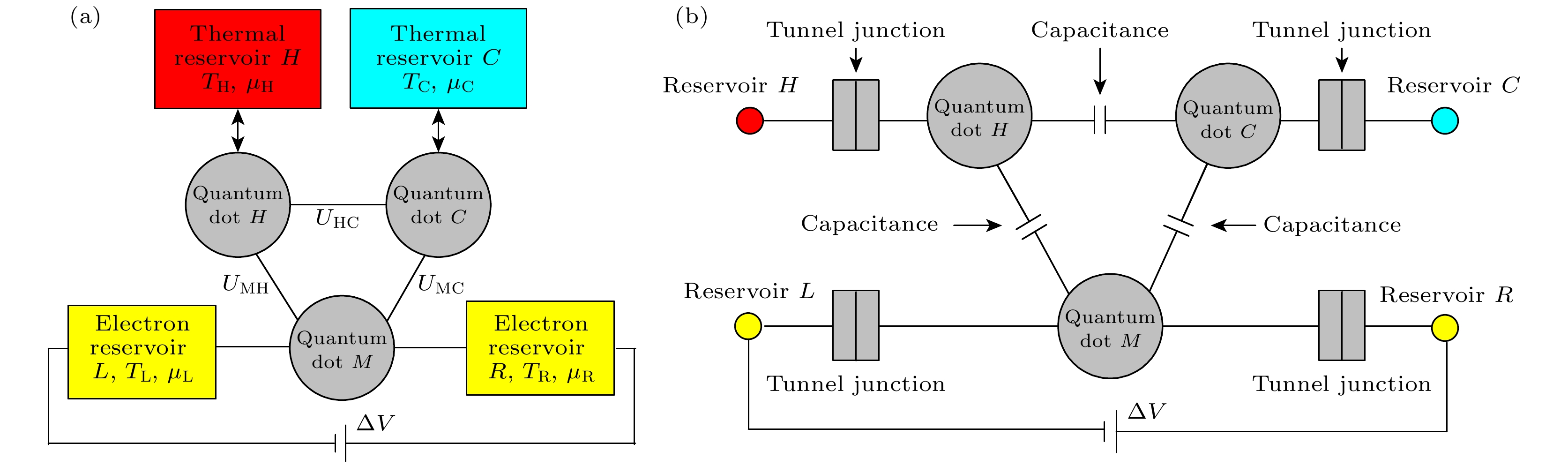
图 1 (a) 基于三量子点耦合的四端制冷机的示意图; (b) (a)中装置的等效电路图

Fig. 1. (a) Schematic diagram of a four terminal refrigerator based on three coupled quantum dots, and (b) is the equivalent circuit diagram of the device in (a).

下载: 全尺寸图片幻灯片

图 2 图1描述的八种量子态的跃迁过程

Fig. 2. The transition processes of eight quantum states described in Fig. 1.

下载: 全尺寸图片幻灯片

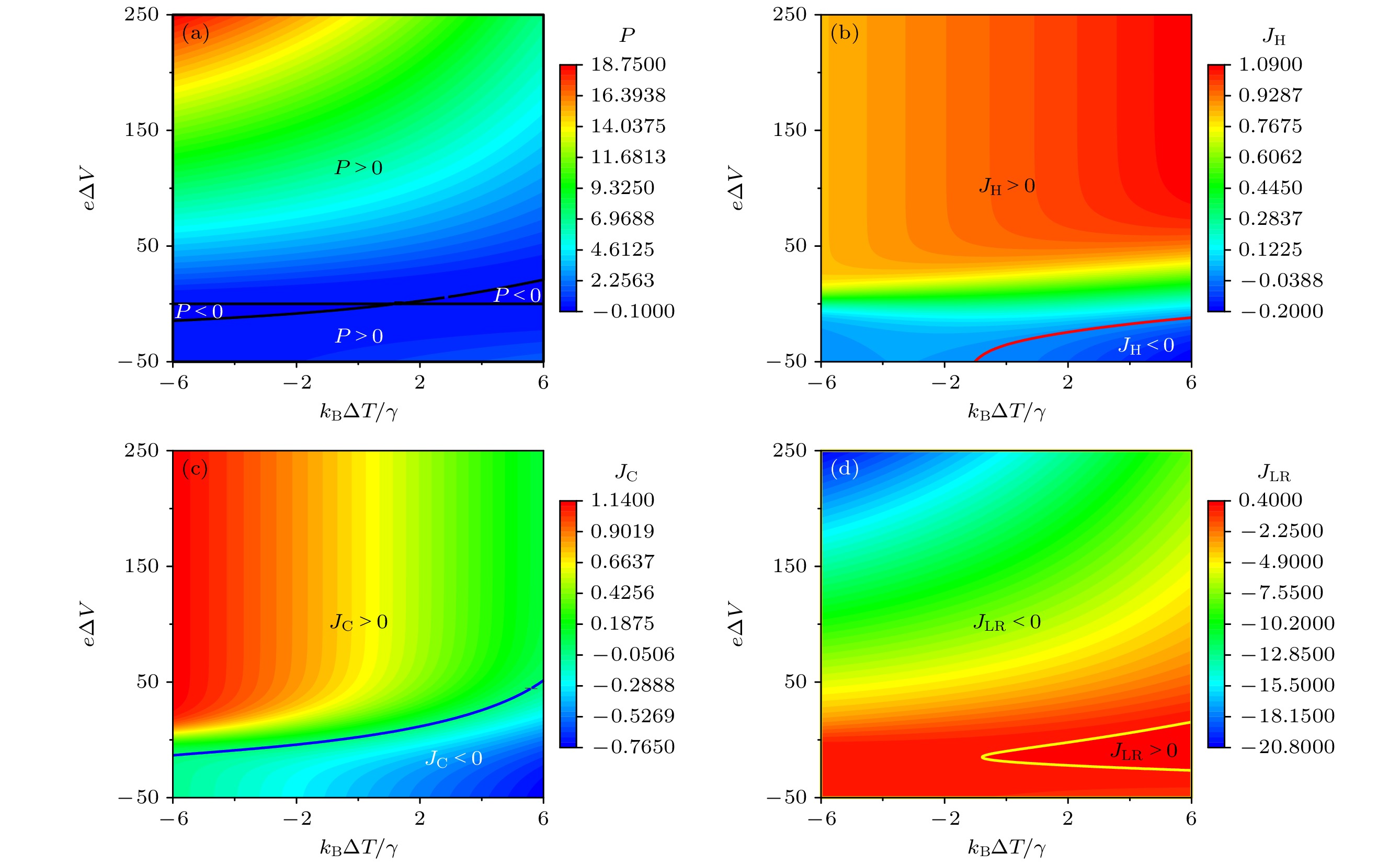
图 3 当耗散系数为$ \lambda = 0 $时,　(a) 输入功率$ P $以及(b)—(d)各量子点与对应库之间的热流J_H, J_C, J_LR随温差$ \Delta T $和偏置电压$ e\Delta V $变化的三维投影图

Fig. 3. The three-dimensional projection graphs for (a) input power $ P $ and (b)–(d) the heat flow J_H, J_C, J_LR varying with the temperature difference $ \Delta T $ and the bias voltage $ e\Delta V $ under the dissipation factor $ \lambda = 0 $.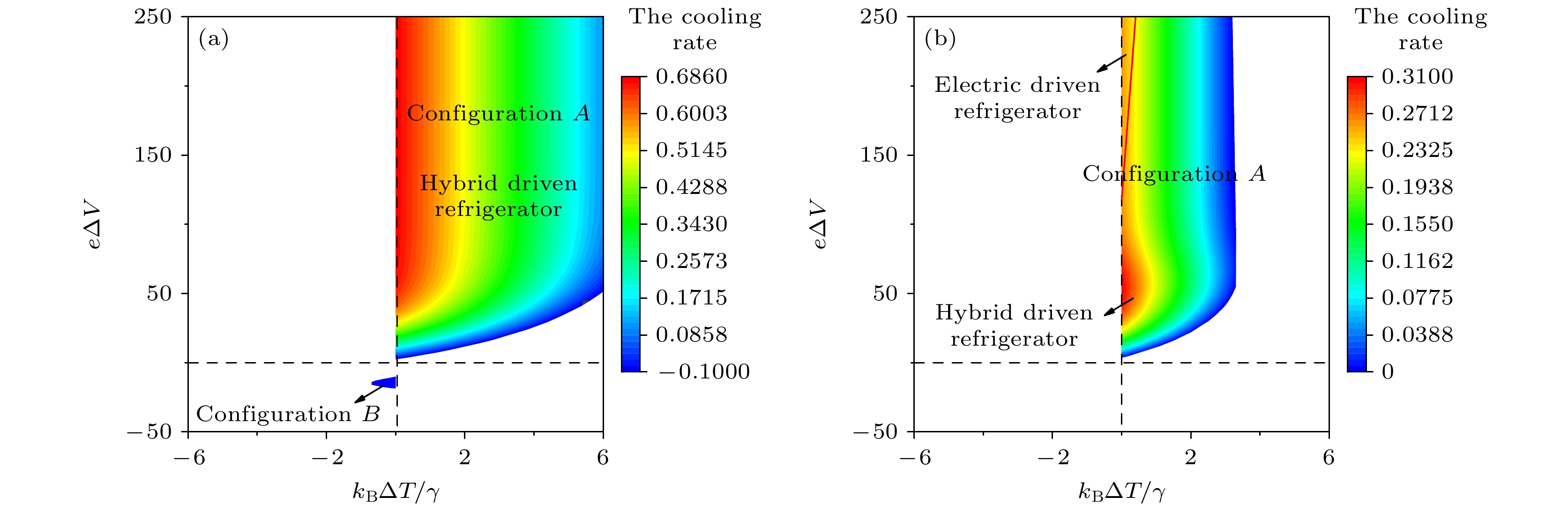

下载: 全尺寸图片幻灯片

图 4 当耗散系数为$ \lambda = 0 $和$ \lambda = 0.26 $时, 装置A和装置B各自对应的工作区域

Fig. 4. The corresponding working areas of device A and device B when the dissipation factor is (a) $ \lambda = 0 $ and (b) $ \lambda = 0.26 $, respectively.

下载: 全尺寸图片幻灯片

图 5 在不同耗散系数下, 装置作为混合驱动制冷机时的总熵产率随温差$ \Delta T $和偏置电压$ e\Delta V $变化的三维曲线

Fig. 5. The three-dimensional curves of total entropy production rate varying with temperature difference $ \Delta T $ and bias voltage $ e\Delta V $ when the device is used as a hybrid-driven refrigerator under different dissipation factor.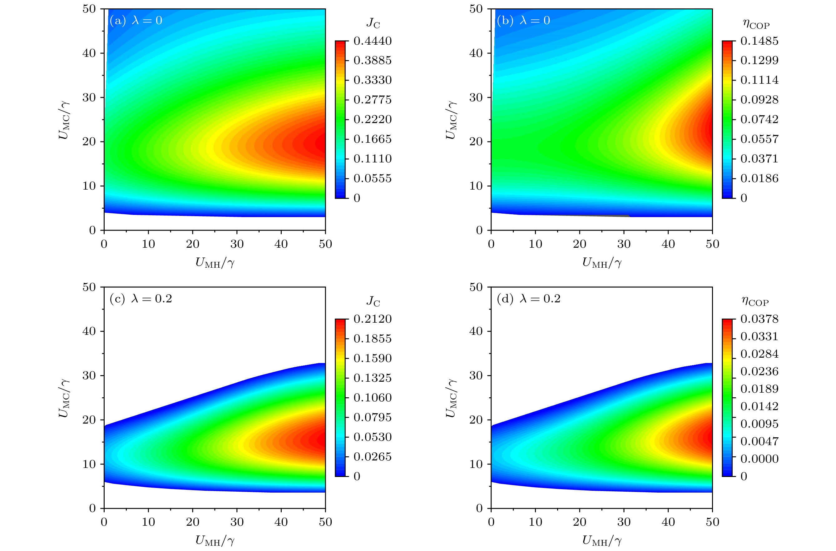

下载: 全尺寸图片幻灯片

图 6 在不同耗散系数下, 制冷率和制冷系数随充电能$ {U_{{\text{MH}}}} $和$ {U_{{\text{MC}}}} $变化的三维图

Fig. 6. The three-dimensional diagrams of the cooling rate and the COP varying with charging energy $ {U_{{\text{MH}}}} $ and $ {U_{{\text{MC}}}} $ under different dissipation factor.

下载: 全尺寸图片幻灯片

图 7 在不同的耗散系数下, 制冷率和制冷系数随充电能$ {U_{{\text{MH}}}} $和偏置电压$ eV $变化的三维图

Fig. 7. The three-dimensional diagrams of the cooling rate and the COP varying with charging energy $ {U_{{\text{MH}}}} $ and bias voltage $ e\Delta V $ under different dissipation factor.

下载: 全尺寸图片幻灯片

图 8 在给定条件$ \Delta T = 2\gamma /{k_{\text{B}}} $下,　(a) 优化的制冷率$ {J_{{\text{Copt}}}} $和(b)优化制冷率对应的制冷系数以及(c)对应的充电能$ {U_{{\text{MC}}}} $随耗散系数$ \lambda $的变化曲线

Fig. 8. The curves of (a) the optimized cooling rate $ {J_{{\text{Copt}}}} $ and (b) the COP corresponding to optimized cooling rate and (c) the corresponding charging energy $ {U_{{\text{MC}}}} $ as a function of dissipation factor $ \lambda $ under the given condition $ \Delta T = 2\gamma /{k_{\text{B}}} $.

下载: 全尺寸图片幻灯片

图 9 (a) 最大制冷率$ {J_{{\text{C}}\max }} $和最大制冷率对应的COP$ {\eta _{\text{J}}} $; (b) 最佳充电能量$ {U_{{\text{MC}}}} $随温差$ \Delta T $的变化曲线

Fig. 9. The curves of (a) the maximum cooling rate $ {J_{{\text{C}}\max }} $ and the COP corresponding to maximum cooling rate $ {\eta _{\text{J}}} $ and (b) the optimal charging energy $ {U_{{\text{MC}}}} $ as a function of temperature difference $ \Delta T $.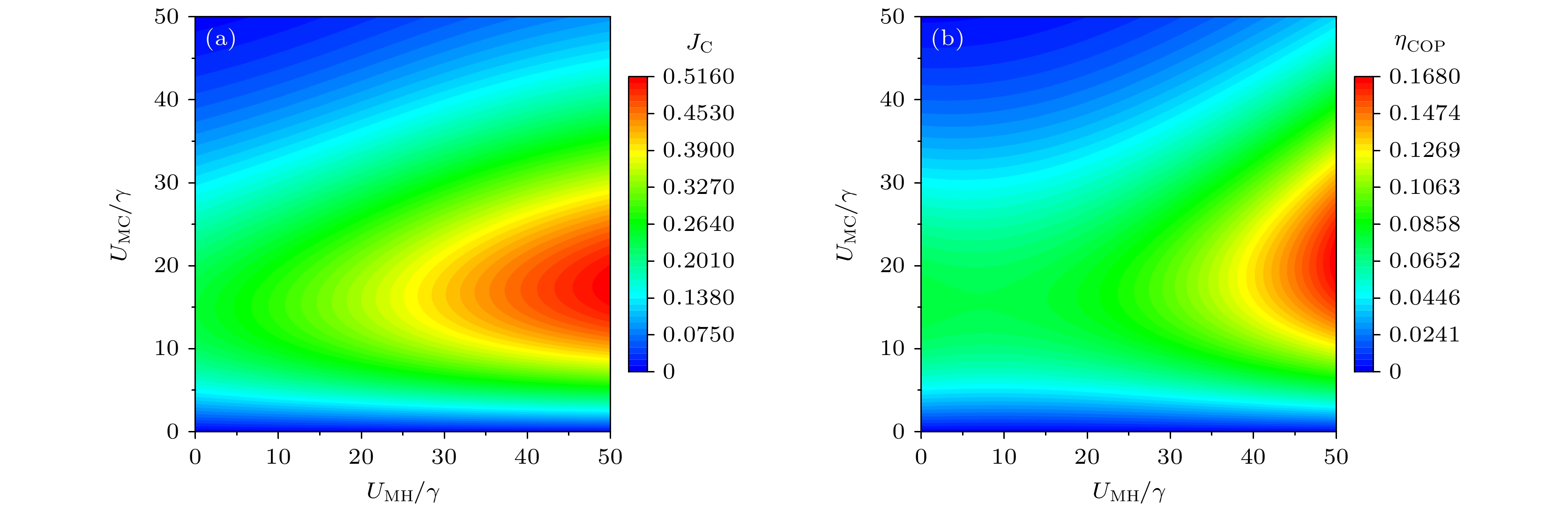

下载: 全尺寸图片幻灯片

图 10 在强耦合$ {U_{{\text{HC}}}} $的情况下, 当$ \lambda = 0 $时,　(a) 制冷率$ {J_{\text{C}}} $和(b)制冷系数$ {\eta _{{\text{COP}}}} $随着$ {U_{{\text{MH}}}} $和$ {U_{{\text{MC}}}} $变化的三维图

Fig. 10. In the case of strong coupling $ {U_{{\text{HC}}}} $, when $ \lambda = 0 $, the three-dimensional diagrams for (a) cooling rate $ {J_{\text{C}}} $ and (b) the COP varying with $ {U_{{\text{MH}}}} $ and $ {U_{{\text{MC}}}} $.

下载: 全尺寸图片幻灯片

[1]	Chen L, Ding Z, Sun F 2011 Energy 36 4011 Google Scholar
[2]	Sánchez R, Büttiker M 2011 Phys. Rev. B 83 085428 Google Scholar
[3]	Thierschmann H, Sánchez R, Sothmann B, Arnold F, Heyn C, Hansen W, Buhmann H, Molenkamp L W 2015 Nat. Nanotechnol 10 854 Google Scholar
[4]	Zhang Y C, Lin G X, Chen J C 2015 Phys. Rev. E 91 052118 Google Scholar
[5]	Zhang Y C, Huang C K, Lin G X, Chen J C 2015 Energy 85 200 Google Scholar
[6]	Zhang Y C, Wang Y, Huang C K, Lin G X, Chen J C 2016 Energy 95 593 Google Scholar
[7]	Aniket S. 2020 J. Appl. Phys 127 234903 Google Scholar
[8]	Anamika B, Surojit H, Shailendra K, Varshney, Gourab D, Aniket S 2021 Phys. Rev. E 103 012131 Google Scholar
[9]	Kano S, Fujii M 2017 Nanotechnology 28 095403 Google Scholar
[10]	Lim J S, Sánchez D, López R 2018 N. J. Phys. 20 023038 Google Scholar
[11]	Daré A M, Lombardo P 2017 Phys. Rev. B 96 115414 Google Scholar
[12]	Su H, Shi Z C, He J Z 2015 Chin. Phys. Lett. 32 100501 Google Scholar
[13]	苏豪, 王家伟, 赵沁园, 何济洲 2016 中国科学: 技术科学 46 1296 Google Scholar Su H, Wang J W, Zhao Q Y, He J Z 2016 Sci. Sin-Tech. 46 1296 Google Scholar
[14]	Shi Z C, Qin W F, He J Z 2016 Mod. Phys. Lett. B 30 1650397 Google Scholar
[15]	Roche B, Roulleau P, Jullien T, Jompol, Y, Farrer I, Ritchie D A, Glattli D C. 2015 Nat. Commun 6 6738 Google Scholar
[16]	Hartmann F, Pfeffer P, Höfling S, Kamp M, Worschech L. 2015 Phys. Rev. Lett. 114 146805 Google Scholar
[17]	Josefsson M, Svilans A, Burke A, Hoffmann E, Fahlvik S, Thelander C, Leijnse M, Linke H 2018 Nat. Nanotechnol 13 920 Google Scholar
[18]	Keller A J, Lim J S, Sánchez D, López R, Amasha S, Katine J A 2016 Phys. Rev. Lett. 117 066602 Google Scholar
[19]	Sothmann B, Sánchez R, Jordan A N, Büttiker M 2013 N. J. Phys. 15 095021 Google Scholar
[20]	Choi Y, Jordan A N 2015 Physica E:Low-dimensional Systems Nanostruct 74 465 Google Scholar
[21]	Lin Z B, Yang Y Y, Fu J, Li W, He J Z 2019 Chin. Phys. Lett. 36 060501 Google Scholar
[22]	Lin Z B, Li W, Yang Y Y, He J Z 2020 Phys. Rev. E 101 022117 Google Scholar
[23]	Sothmann B, Sánchez R, Jordan A N 2014 Europhys. Lett. 107 47003 Google Scholar
[24]	Sánchez R, Sothmann B, Jordan A N 2015 Phys. Rev. Lett. 114 146801 Google Scholar
[25]	Boukai A I, Bunimovich Y, Tahir-Kheli J, Yu J K, Goddard I W A, Heath J R 2008 Nature 451 168 Google Scholar
[26]	Yang Y Y, Xu S, Li W, He J Z 2020 Phys. Scr. 95 095001 Google Scholar
[27]	Yang Y Y, Xu S, He J Z 2020 Chin. Phys. Lett. 37 120502 Google Scholar
[28]	Su S, Zhang Y, Chen J, Shih T M 2016 Sci. Reports 6 21425 Google Scholar
[29]	Shi Z C, Fu J, Qin W F, He J Z 2017 Chin. Phys. Lett. 34 110501 Google Scholar
[30]	Jiang J H, Entin-Wohlman O, Imry Y 2013 New Journal of Physics 15 075021 Google Scholar
[31]	Li C, Zhang Y, He J 2013 Chin. Phys. Lett. 30 100501 Google Scholar
[32]	Rutten B, Esposito M, Cleuren B 2009 Phys. Rev. B 80 235122 Google Scholar
[33]	Cleuren B, Rutten B, Van den Broeck C 2012 Phys. Rev. Lett. 108 120603 Google Scholar
[34]	施志诚, 何济洲, 肖宇玲 2015 中国科学: 物理学力学天文学 45 050502 Google Scholar Shi Z C, He J Z, Xiao Y L 2015 Sci. Sin-Phys. Mech. Astron. 45 050502 Google Scholar
[35]	Li C, Zhang Y, Wang J, He J 2013 Phys. Rev. E 88 062120 Google Scholar
[36]	Wang J H, Lai Y M, Ye Z L, He J Z, Ma Y L, Liang Q H 2015 Phys. Rev. E 91 050102 Google Scholar
[37]	李唯, 符婧, 杨贇贇, 何济洲 2019 物理学报 68 220501 Google Scholar Li W, Fu J, Yang Y Y, He J Z 2019 Acta Phys. Sin. 68 220501 Google Scholar
[38]	Whitney R S, Sánchez R, Haupt F, Splettstoesser J 2016 Phys. E 82 176 Google Scholar
[39]	Fu T, Du J Y, Su S H, Su G Z, Chen J C 2021 Eur. Phys. J. Plus 136 1059 Google Scholar
[40]	Xi M M, Wang R Q, Lu J C, Chen T Y, Jiang J H 2021 Chin. Phys. Lett 38 088801 Google Scholar
[41]	苏山河, 张艳超, 彭万里, 苏国珍, 陈金灿 2021 中国科学: 物理学力学天文学 51 112 Google Scholar Su S H, Zhang Y C, Peng W L, Su G Z, Chen J C 2021 Sci. Sin-Phys. Mech. Astron. 51 112 Google Scholar

[1]	刘旭明, 查奎帆, 马帅, 韩丽明, 谢晓霖, 郭伟杰, 潘长钊. 基于脉管制冷机预冷的1K大冷量低温系统. 物理学报, 2025, 74(11): . doi: 10.7498/aps.74.20250181
[2]	郑茂文, 郭浩文, 卫铃佼, 潘子杰, 邹佳润, 李瑞鑫, 赵密广, 陈厚磊, 梁惊涛. 稀释制冷技术. 物理学报, 2024, 73(23): 230701. doi: 10.7498/aps.73.20241211
[3]	李珂, 王亚男, 刘萍, 禹芳秋, 戴巍, 沈俊. 50 mK多级绝热去磁制冷机的实验研究. 物理学报, 2023, 72(19): 190702. doi: 10.7498/aps.72.20231102
[4]	刘旭明, 潘长钊, 张宇, 廖奕, 郭伟杰, 俞大鹏. 4 K大冷量GM型脉冲管制冷机. 物理学报, 2023, 72(19): 190701. doi: 10.7498/aps.72.20230910
[5]	俎红叶, 程维军, 王亚男, 王晓涛, 李珂, 戴巍. 冷凝泵型稀释制冷机实验研究. 物理学报, 2023, 72(8): 080701. doi: 10.7498/aps.72.20222257
[6]	徐帅, 杨贇贇, 刘行, 何济洲. 基于一维弹道导体的三端纳米线制冷机的性能优化. 物理学报, 2022, 71(2): 020501. doi: 10.7498/aps.71.20211077
[7]	王昌, 李珂, 沈俊, 戴巍, 王亚男, 罗二仓, 沈保根, 周远. 用于亚开温区的极低温绝热去磁制冷机. 物理学报, 2021, 70(9): 090702. doi: 10.7498/aps.70.20202237
[8]	付柏山, 廖奕, 周俊. 稀释制冷机及其中的热交换问题. 物理学报, 2021, 70(23): 230202. doi: 10.7498/aps.70.20211760
[9]	李唯, 符婧, 杨贇贇, 何济洲. 光子驱动量子点制冷机. 物理学报, 2019, 68(22): 220501. doi: 10.7498/aps.68.20191091
[10]	张荣, 卢灿灿, 李倩文, 刘伟, 白龙. 线性不可逆热力学框架下一个无限尺寸热源而有限尺寸冷源的制冷机的性能分析. 物理学报, 2018, 67(4): 040502. doi: 10.7498/aps.67.20172010
[11]	李振兴, 李珂, 沈俊, 戴巍, 高新强, 郭小惠, 公茂琼. 室温磁制冷技术的研究进展. 物理学报, 2017, 66(11): 110701. doi: 10.7498/aps.66.110701
[12]	高新强, 沈俊, 和晓楠, 唐成春, 戴巍, 李珂, 公茂琼, 吴剑峰. 耦合高压斯特林制冷效应的复合磁制冷循环的数值模拟. 物理学报, 2015, 64(21): 210201. doi: 10.7498/aps.64.210201
[13]	崔尉, 王茺, 崔灿, 施张胜, 杨宇. 耦合锗量子点中空穴态对称特性研究. 物理学报, 2014, 63(22): 227301. doi: 10.7498/aps.63.227301
[14]	汤乃云. 耦合量子点中空穴基态反键态特性研究. 物理学报, 2013, 62(5): 057301. doi: 10.7498/aps.62.057301
[15]	何弦, 何济洲, 肖宇玲. 四能级量子制冷循环. 物理学报, 2012, 61(15): 150302. doi: 10.7498/aps.61.150302
[16]	贺兵香, 何济洲, 缪贵玲. 纳米线异质结构对电子制冷机性能的影响. 物理学报, 2011, 60(4): 040509. doi: 10.7498/aps.60.040509
[17]	贺兵香, 何济洲. 双势垒InAs/InP纳米线异质结热电子制冷机. 物理学报, 2010, 59(6): 3846-3850. doi: 10.7498/aps.59.3846
[18]	谌雄文, 谌宝菊, 施振刚, 宋克慧. 嵌入T型耦合双量子点介观A-B环系统的显著Fano 效应. 物理学报, 2009, 58(4): 2720-2725. doi: 10.7498/aps.58.2720
[19]	谌雄文, 贺达江, 吴绍全, 宋克慧. 嵌入平行量子点的非平衡介观环路的极化电流. 物理学报, 2006, 55(8): 4287-4291. doi: 10.7498/aps.55.4287
[20]	吴绍全, 谌雄文, 孙威立, 王顺金. 嵌入耦合量子点的介观Aharonov-Bohm环内的持续电流. 物理学报, 2004, 53(7): 2336-2341. doi: 10.7498/aps.53.2336

计量

文章访问数: 4713
PDF下载量: 72
被引次数: 0

姓名
邮箱
手机号码
标题
留言内容
验证码

搜索

留言板

基于三个耦合量子点的四端混合驱动制冷机