


-
在就地γ谱仪搜索扫描测量“热粒子”、“放射性汇集点”、“放射性汇集区”过程中, 只能给出污染源的大概位置, 不能给出源的污染深度等边界参数. 本文主要对虚拟技术在就地γ谱仪搜索扫描测量细化污染源边界中的应用进行了研究. 将就地γ谱仪测量对象简化成衰减层 + 放射性热区(测量目标源) + 衰减层 + 干扰源的四层理论模型, 运用虚拟技术将源项层虚拟成点源, 进一步简化了理论模型, 使用蒙特卡罗方法模拟计算探测效率与峰谷比等参数, 最后使用最小二乘法使模拟计算结果反演逼近源项实际参数, 从而建立了源边界参数反演计算的理论方法及步骤. 理论研究和实验结果一致, 验证了所建立的计算模型和技术方法是正确可靠的. 目前, 对于均匀分布的放射性核素, 该技术已经能够准确确定污染区域深度分布等边界参数, 从而在治理时达到废物处置减容的目的. 同时, 该技术对于禁核试核查目标核弹头惰层厚度参数的确定也具有重大的参考价值.In the in situ γ spectrometer based measurement of " hot particular”, " radioactive collection point” and " radioactive collection area”, only the position of the pollution source can be located roughly, but its boundary parameters such as the thickness of pollution source cannot be given. In this paper, the application of virtual technology to the scanning of γ spectrometer is studied. We convert γ spectrometer measurement objects into a four-layer theoretical model, which are attenuation thickness + radioactive hot area + attenuation thickness + disturb source. Then, the source item layer is virtualized into a point source by using virtual technology. So, the theoretical model is further simplified. Then the detection efficiency and peak/valley ratio parameter of source term are simulated by Monte Carlo method. Finally, the source term parameters are retrieved by using the least square method, and thus establishing the theoretical method and procedure of inversion calculation of source boundary parameters. In this paper, the theoretical and experimental results are shown to be consistent with each other. So, this method is verified to be correct and practicable. Currently, the method can accurately determine the depth distribution parameters of radioactive contamination area for uniformly distributed radio nuclides. In conclusion, the technical achievements can be used to accurately determine the boundary range of the radioactive hot zone, thus realizing the purpose of reducing the waste disposal capacity during the treatment. At the same time, the determination of the inert layer thickness parameters of the target nuclear warhead of Nuclear Test Ban Treaty has a significant reference value.
-
Keywords:
- virtual point source /
- parameter characterization /
- Monte Carlo simulation /
- source boundary
[1] 熊宗华, 亢武, 龚建, 胡广春, 向永春, 裴永全 2003 物理学报 52 1
 Google Scholar
Xiong Z H, Kang W, Gong J, Hu G C, Xiang Y C, Pei Y Q 2003 Atca Phys. Sin. 52 1
Google Scholar
[2] Kováik A, Sy′kora I, Povinec P P 2013 J. Radioanal. Nucl. Chem. 298 665
Google Scholar
[3] Peyres V, García-Torao E 2007 Nucl. Instr. Meth. Phys. Res. A 580 296
Google Scholar
[4] 田自宁, 欧阳晓平, 殷经鹏, 张洋, 杨文静 2013 原子能科学技术 47 1411
Google Scholar
Tian Z N, Ouyang X P, Yin J P, Zhang Y, Yang W J 2013 Atomic Energy Sci. Technol. 47 1411
Google Scholar
[5] Elanique A, Marzocchi O, Leone D, Hegenbart L, Breustedt B, Oufni L 2012 Appl. Radiat. Isot. 70 538
Google Scholar
[6] Budjá D, Heisel M, Maneschg W, Simgen H 2009 Appl. Radiat. Isot. 67 706
Google Scholar
[7] Gasparro J, Hult M, Johnston P N, Tagziria H 2008 Nucl. Instr. Meth. Phys. Res. A 594 196
Google Scholar
[8] Huya N Q, Binhb D Q, An V X 2007 Nucl. Instr. Meth. Phys. Res. A 573 384
Google Scholar
[9] Huy N Q 2010 Nucl. Instr. Meth. Phys. Res. A 621 390
Google Scholar
[10] Luís R, Bento J, Carvalhal G, Nogueira P, Silva L, Teles P, Vaz P 2010 Nucl. Instr. Meth. Phys. Res. A 623 1014
Google Scholar
[11] Mohammadi M A, Abdi M R, Kamali M, Mostajaboddavati M, Zare M R 2011 Appl. Radiat. Isot. 69 521
Google Scholar
[12] Presler O, German U, Pelled O, Alfassi Z B 2004 Appl. Radiat. Isot. 60 213
Google Scholar
[13] Mahling S, Orion I, Alfassi Z B 2006 Nucl. Instr. Meth. Phys. Res. A 557 544
Google Scholar
[14] 熊文彬, 仇春华, 段天英, 刘浩杰, 潘君艳, 陈海涛, 刘进辉 2011 原子能科学技术 45 999
Xiong W B, Qiu C H, Duan T Y, Liu H J, Pan J Y, Chen H T, Liu J H 2011 Atomic Energy Sci. Technol. 45 999
[15] Noteal A 1971 Nucl. Instr. Meth. 91 513
Google Scholar
[16] 田自宁, 欧阳晓平, 曾鸣, 成智威 2013 物理学报 62 162902
Google Scholar
Tian Z N, Ouyang X P, Zeng M, Cheng Z W 2013 Acta Phys. Sin. 62 162902
Google Scholar
[17] 田自宁, 陈伟, 韩斌, 田言杰, 刘文彪, 冯天成, 欧阳晓平 2016 物理学报 65 062901
Google Scholar
Tian Z N, Chen W, Han B, Tian Y J, Liu W B, Feng T C, Ouyang X P 2016 Acta Phys. Sin. 65 062901
Google Scholar
-
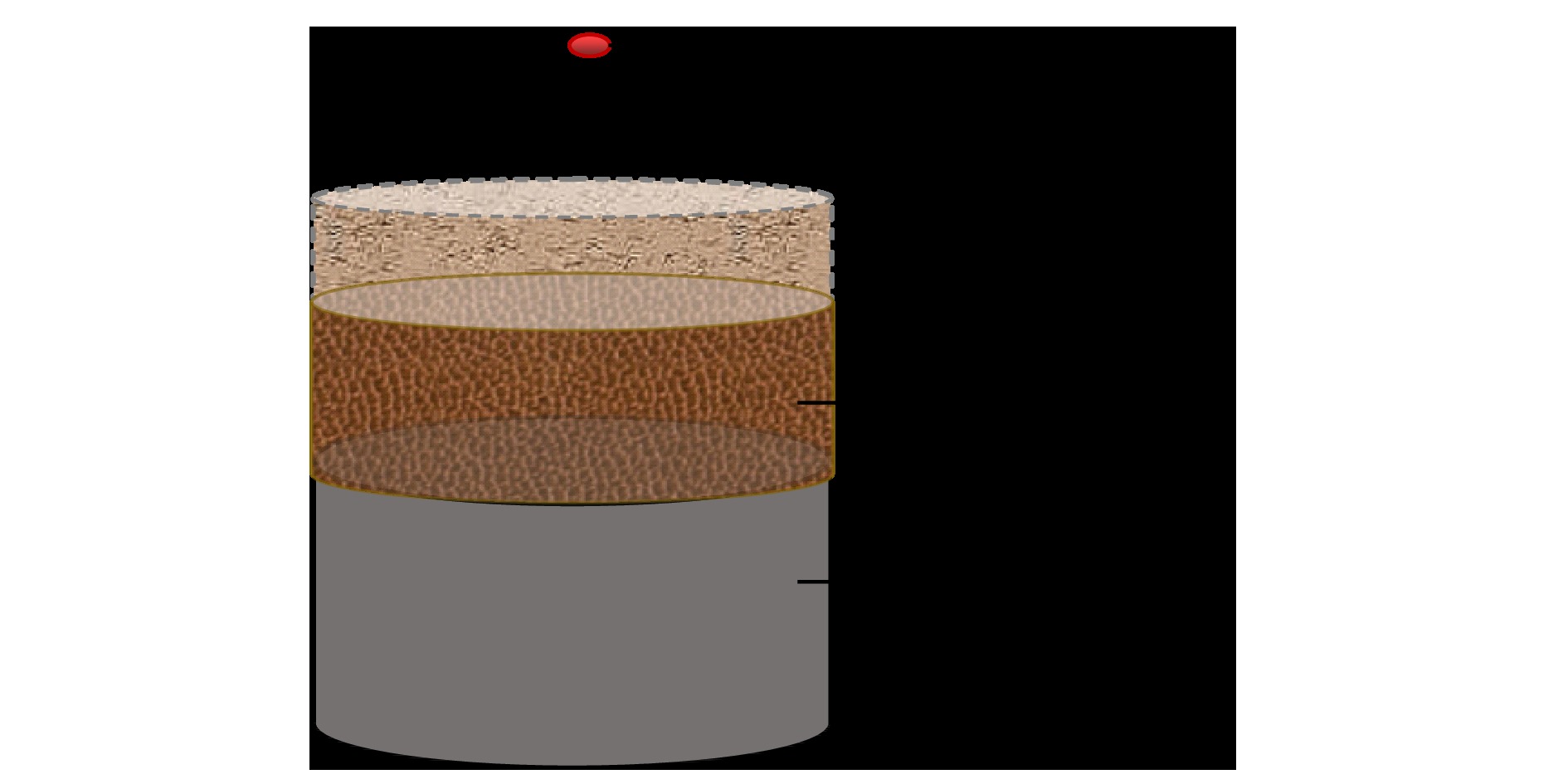
图 4 探测模式1的MCNP程序计算模型
Fig. 4. Calculation model of MCNP procedure for detection mode 1.
图 5 探测模式2的MCNP程序计算模型
Fig. 5. Calculation model of MCNP procedure for detection mode 2.
表 1 探测模式1实验能谱峰计数及处理结果
Table 1. Energy peak count of experimental spectrum and process results for detection mode 1.
测量对象 测量时长t/105 s N241 (54—57 keV) N241 (59.54 keV) N239 (51.62, 129 keV) A/104 Bq 241Am 239Pu 探测模式1 3.16 4325136 25339979 — — — 239Pu体源 2.00 — 75248200 239711, 52717 4.56 18.7  下载: 导出CSV
表 2 探测模式2实验能谱峰计数及处理结果
Table 2. Energy peak count of experimental spectrum and process results for detection mode 2.
测量对象 测量时长 t/105 s N241 (26.4 keV) N241 (54—57 keV) N241 (59.54 keV) A/× 104 Bq 26.4 keV 59.54 keV 探测模式2 4.00 240050 9531180 65964536 8.16 8.91 241Am点源 0.565 4160024 — 65331456 7.74 8.38 241Am体源 0.800 45346 — 2745773 0.423 0.532
下载: 导出CSV
表 3 等效虚拟点源探测效率及峰谷比
Table 3. The detection efficiency and peak/valley of equivalent virtual point source.
h/cm ${\varepsilon _{241}}(h)$/10–3 ${\varepsilon _{239}}(h)$/10–3 A241/104 Bq A239/105 Bq Q ${N}/{ { {N_{\rm v}} } }(h)$ –1.25 24.3 24.6 0.921 0.497 5.4 8.05 –1.60 17.9 19.5 1.24 0.629 5.0 6.99 –2.00 12.9 15.1 1.73 0.810 4.7 6.12 –2.40 9.45 11.9 2.36 1.03 4.4 5.44 –2.80 7.00 9.45 3.19 1.30 4.1 4.92 –3.20 5.24 7.60 4.26 1.61 3.8 4.51 –3.60 3.97 6.16 5.62 1.98 3.5 4.18 –3.80 3.47 5.56 6.45 2.20 3.4 4.04 –4.00 3.03 5.04 7.37 2.43 3.3 3.90
下载: 导出CSV
表 4 不同组合下等效虚拟点的均方偏差计算数据
Table 4. The mean square deviation calculation data of equivalent virtual point at different combination.
w h/cm $\varepsilon (h)$/10–3 ${\varepsilon ^*}(h)$/10–3 ${N}/{ { {N_{\rm v}} } }(h)$ X2/10–3 X3/10–3 X1 $\sigma (X)$ 0.10 –1.25 24.3 24.6 8.05 — — — — 0.90 –3.20 5.24 7.60 4.51 7.15 9.30 4.87 0.177 0.90 –3.60 3.97 6.16 4.18 6.00 8.01 4.56 0.308 0.90 –3.80 3.47 5.56 4.04 5.55 7.47 4.44 0.385 0.90 –4.00 3.03 5.04 3.90 5.16 6.99 4.31 0.458 0.10 –1.60 17.9 19.5 6.99 — — — — 0.90 –3.20 5.24 7.60 4.51 6.51 8.79 4.76 0.217 0.90 –3.60 3.97 6.16 4.18 5.36 7.50 4.46 0.396 0.90 –3.80 3.47 5.56 4.04 4.91 6.96 4.33 0.479 0.90 –4.00 3.03 5.04 3.90 4.52 6.48 4.21 0.554 0.10 –2.00 12.9 15.1 6.12 — — — — 0.90 –3.20 5.24 7.60 4.51 6.01 8.35 4.67 0.277 0.90 –3.60 3.97 6.16 4.18 4.86 7.06 4.37 0.474 0.90 –3.80 3.47 5.56 4.04 4.41 6.52 4.24 0.559 0.90 –4.00 3.03 5.04 3.90 4.02 6.04 4.12 0.635 0.10 –2.40 9.45 11.9 5.44 — — — — 0.90 –3.20 5.24 7.60 4.51 5.66 8.03 4.61 0.327 0.90 –3.60 3.97 6.16 4.18 4.52 6.74 4.30 0.530 0.90 –3.80 3.47 5.56 4.04 4.06 6.20 4.18 0.616 0.90 –4.00 3.03 5.04 3.90 3.67 5.72 4.05 0.693
下载: 导出CSV
表 5 不同组合下等效虚拟点的均方偏差计算数据
Table 5. The mean square deviation calculation data of equivalent virtual point at different combination.
h/cm w $\sigma (X)$ w $\sigma (X)$ w $\sigma (X)$ w $\sigma (X)$ w $\sigma (X)$ –1.25 0.10 — 0.20 — 0.30 — 0.40 — 0.50 — –3.20 0.90 0.177 0.80 0.355 0.70 0.664 0.60 0.988 0.50 1.32 –3.60 0.90 0.308 0.80 0.223 0.70 0.508 0.60 0.848 0.50 1.20 –3.80 0.90 0.385 0.80 0.201 0.70 0.448 0.60 0.792 0.50 1.15 –4.00 0.90 0.458 0.80 0.210 0.70 0.399 0.60 0.744 0.50 1.11 –1.60 0.10 — 0.20 — 0.30 — 0.40 — 0.50 — –3.20 0.90 0.217 0.80 0.195 0.70 0.360 0.60 0.568 0.50 0.784 –3.60 0.90 0.396 0.80 0.210 0.70 0.234 0.60 0.435 0.50 0.669 –3.80 0.90 0.479 0.80 0.262 0.70 0.203 0.60 0.384 0.50 0.622 –4.00 0.90 0.554 0.80 0.318 0.70 0.196 0.60 0.343 0.50 0.583 –2.00 0.10 — 0.20 — 0.30 — 0.40 — 0.50 — –3.20 0.90 0.277 0.80 0.187 0.70 0.177 0.60 0.256 0.50 0.371 –3.60 0.90 0.474 0.80 0.328 0.70 0.210 0.60 0.181 0.50 0.272 –3.80 0.90 0.559 0.80 0.399 0.70 0.257 0.60 0.178 0.50 0.238 –4.00 0.90 0.635 0.80 0.465 0.70 0.307 0.60 0.193 0.50 0.215 –2.40 0.10 — 0.20 — 0.30 — 0.40 — 0.50 — –3.20 0.90 0.327 0.80 0.264 0.70 0.209 0.60 0.173 0.50 0.167 –3.60 0.90 0.530 0.80 0.435 0.70 0.344 0.60 0.261 0.50 0.195 –3.80 0.90 0.616 0.80 0.510 0.70 0.407 0.60 0.309 0.50 0.225 –4.00 0.90 0.693 0.80 0.577 0.70 0.464 0.60 0.356 0.50 0.257
下载: 导出CSV
h/cm w $\sigma (X)$ w $\sigma (X)$ w $\sigma (X)$ w $\sigma (X)$ –1.25 0.60 — 0.70 — 0.80 — 0.9 — –3.20 0.40 1.65 0.30 1.98 0.20 2.31 0.10 2.64 –3.60 0.40 1.55 0.30 1.90 0.20 2.26 0.10 2.61 –3.80 0.40 1.51 0.30 1.88 0.20 2.24 0.10 2.60 –4.00 0.40 1.48 0.30 1.85 0.20 2.22 0.10 2.60 –1.60 0.60 — 0.70 — 0.80 — 0.90 — –3.20 0.40 1.00 0.30 1.23 0.20 1.45 0.10 1.67 –3.60 0.40 0.910 0.30 1.16 0.20 1.40 0.10 1.65 –3.80 0.40 0.872 0.30 1.13 0.20 1.38 0.10 1.64 –4.00 0.40 0.839 0.30 1.10 0.20 1.37 0.10 1.63 –2.00 0.60 — 0.70 — 0.80 — 0.90 — –3.20 0.40 0.498 0.30 0.630 0.20 0.763 0.10 0.898 –3.60 0.40 0.410 0.30 0.561 0.20 0.716 0.10 0.875 –3.80 0.40 0.375 0.30 0.533 0.20 0.698 0.10 0.865 –4.00 0.40 0.347 0.30 0.509 0.20 0.681 0.10 0.857 –2.40 0.60 — 0.70 — 0.80 — 0.90 — –3.20 0.40 0.194 0.30 0.244 0.20 0.305 0.10 0.372 –3.60 0.40 0.169 0.30 0.199 0.20 0.267 0.10 0.351 –3.80 0.40 0.174 0.30 0.186 0.20 0.252 0.10 0.342 –4.00 0.40 0.186 0.30 0.178 0.20 0.240 0.10 0.335
下载: 导出CSV
表 6 体源参数的反演计算数据
Table 6. The inversion data of volume source parameters.
hV/cm 体源厚度/cm $\varepsilon ({h_{\rm{V}}})$
/10–3${\varepsilon ^*}({h_{\rm{V}}})$
/10–2${N}/{ { {N_{\rm v}} } }({h_{\rm{V} } })$ $\sigma (X)$ –2.80 0.80 4.54 0.689 4.69 0.444 –2.80 1.2 4.60 0.696 4.74 0.431 –2.80 1.6 4.70 0.705 4.81 0.414 –2.45 0.80 5.68 0.818 5.03 0.231 –2.45 1.2 5.76 0.826 5.07 0.217 –2.45 1.6 5.89 0.837 5.16 0.200 –2.45 2.0 6.05 0.851 5.26 0.181 –2.45 2.5 6.31 0.874 5.41 0.159 –2.45 3.0 6.65 0.903 5.63 0.163 –2.45 4.0 7.57 0.981 6.24 0.289 –2.45 4.9 8.78 1.08 7.12 0.539 –2.00 0.80 7.62 1.03 5.58 0.188 –2.00 1.2 7.75 1.04 5.64 0.212 –2.00 1.6 7.93 1.05 5.75 0.248 –2.00 2.0 8.17 1.07 5.88 0.295 –2.00 2.5 8.55 1.10 6.11 0.373 –2.00 3.0 9.03 1.14 6.41 0.474 –2.00 4.0 10.4 1.25 7.35 0.769 –1.50 0.80 10.7 1.33 6.43 0.744 –1.50 1.2 10.9 1.35 6.54 0.781 –1.50 1.6 11.2 1.37 6.68 0.834 –1.50 2.0 11.5 1.40 6.90 0.905 –1.50 3.0 12.9 1.50 7.79 1.18 –0.50 0.80 22.0 2.34 10.1 2.81
下载: 导出CSV
表 7 等效虚拟点源探测效率、峰谷比及活度比
Table 7. The detection efficiency, peak/valley and acvitiy ratio of equivalent virtual point source.
h/cm ${\varepsilon _{26.4\;{\rm{keV}}}}(h)$/10–3 ${\varepsilon _{59.54\;{\rm{keV}}}}(h)$/10–2 A26.4 keV/104 Bq A59.54 keV/104 Bq A59.54 keV/A26.4 keV ${N}/{ { {N_{\rm v}} } }(h)$ 0.80 48.200 14.4 0.0519 0.318 6.10 17.0 0.40 13.500 8.79 0.1850 0.523 2.80 12.0 0 4.060 5.56 0.6150 0.826 1.30 9.3 –0.20 2.260 4.48 1.1100 1.030 0.90 8.4 –0.40 1.270 3.64 1.9700 1.260 0.60 7.7 –0.60 0.717 2.98 3.4900 1.540 0.40 7.1 –0.80 0.409 2.45 6.1200 1.880 0.30 6.6
下载: 导出CSV
表 9 体源参数的反演计算数据
Table 9. The inversion data of volume source parameters.
hV/cm 体源
厚度/cm${\varepsilon ^*}({h_{\rm{V}}})$/
10–2$\varepsilon ({h_{\rm{V}}})$/
10–3${N}/{ { {N_{\rm v}} } }({h_{\rm{V} } })$ $\sigma (X)$ hV/cm 体源
厚度/cm${\varepsilon ^*}({h_{\rm{V}}})$/
10–2$\varepsilon ({h_{\rm{V}}})$/
10–3${N}/{ { {N_{\rm v}} } }({h_{\rm{V} } })$ $\sigma (X)$ 0.75 1.00 3.54 10.4 11.90 1.5900 0.15 2.20 2.45 5.00 9.34 0.2310 0.75 0.60 3.47 8.06 11.40 1.0100 0.15 1.60 2.31 2.69 8.54 0.3470 0.75 0.30 3.44 7.23 11.20 0.8060 0.15 1.00 2.21 1.72 8.07 0.5920 0.25 2.00 2.59 5.49 9.61 0.3530 0.15 0.40 2.17 1.32 7.86 0.6920 0.25 1.90 2.56 4.91 9.44 0.2110 0 2.50 2.26 4.40 9.00 0.0900 0.25 1.80 2.54 4.42 9.29 0.0890 0 2.45 2.24 4.14 8.90 0.0470 0.25 1.70 2.51 4.00 9.14 0.0220 0 2.40 2.23 3.90 8.83 0.0640 0.25 1.60 2.49 3.63 9.03 0.1090 0 2.00 2.13 2.52 8.30 0.3950 0.25 1.50 2.47 3.32 8.92 0.1870 0 1.50 2.04 1.60 7.83 0.6260 0.25 1.30 2.43 2.81 8.72 0.3130 0 1.00 1.97 1.13 7.54 0.7470 0.25 0.80 2.37 2.04 8.38 0.5080 –0.25 1.10 1.65 0.602 6.86 0.8910 –0.25 0.50 1.61 0.457 6.70 0.9300
下载: 导出CSV
表 8 不同组合下等效虚拟点的均方偏差计算数据
Table 8. The mean square deviation calculation data of equivalent virtual point at different combination.
h/cm w $\sigma (X)$ w $\sigma (X)$ w $\sigma (X)$ w $\sigma (X)$ w $\sigma (X)$ 0.80 0.10 — 0.20 — 0.30 — 0.40 — 0.50 — –0.40 0.90 2.414 0.80 1.783 0.70 2.807 0.60 3.832 0.50 4.86 –0.60 0.90 2.115 0.80 1.512 0.70 2.569 0.60 3.627 0.50 4.69 –0.80 0.90 1.951 0.80 1.362 0.70 2.433 0.60 3.510 0.50 4.59 0.40 0.10 — 0.20 — 0.30 — 0.40 — 0.50 — –0.40 0.90 0.466 0.80 0.291 0.70 0.529 0.60 0.780 0.50 1.03 –0.60 0.90 0.177 0.80 0.119 0.70 0.286 0.60 0.567 0.50 0.857 –0.80 0.90 0.185 0.80 0.245 0.70 0.175 0.60 0.447 0.50 0.753 0 0.10 — 0.20 — 0.30 — 0.40 — 0.50 — –0.40 0.90 0.190 0.80 0.160 0.70 0.168 0.60 0.235 0.50 0.327 –0.60 0.90 0.431 0.80 0.346 0.70 0.214 0.60 0.123 0.50 0.165 –0.80 0.90 0.620 0.80 0.512 0.70 0.350 0.60 0.197 0.50 0.112
下载: 导出CSV
h/cm w $\sigma (X)$ w $\sigma (X)$ w $\sigma (X)$ w $\sigma (X)$ 0.80 0.60 — 0.70 — 0.80 – 0.90 — –0.40 0.40 5.88 0.30 6.91 0.20 7.93 0.10 8.96 –0.60 0.40 5.75 0.30 6.81 0.20 7.87 0.10 8.92 –0.80 0.40 5.67 0.30 6.75 0.20 7.83 0.10 8.90 0.40 0.60 – 0.70 — 0.80 – 0.90 — –0.40 0.40 1.29 0.30 1.55 0.20 1.80 0.10 2.06 –0.60 0.40 1.15 0.30 1.44 0.20 1.73 0.10 2.03 –0.80 0.40 1.06 0.30 1.38 0.20 1.69 0.10 2.01 0 0.60 — 0.70 — 0.80 — 0.90 — –0.40 0.40 0.427 0.30 0.532 0.20 0.639 0.10 0.747 –0.60 0.40 0.287 0.30 0.425 0.20 0.567 0.10 0.711 –0.80 0.40 0.207 0.30 0.361 0.20 0.523 0.10 0.689
下载: 导出CSV
-
[1] 熊宗华, 亢武, 龚建, 胡广春, 向永春, 裴永全 2003 物理学报 52 1
Google Scholar
Xiong Z H, Kang W, Gong J, Hu G C, Xiang Y C, Pei Y Q 2003 Atca Phys. Sin. 52 1
Google Scholar
[2] Kováik A, Sy′kora I, Povinec P P 2013 J. Radioanal. Nucl. Chem. 298 665
Google Scholar
[3] Peyres V, García-Torao E 2007 Nucl. Instr. Meth. Phys. Res. A 580 296
Google Scholar
[4] 田自宁, 欧阳晓平, 殷经鹏, 张洋, 杨文静 2013 原子能科学技术 47 1411
Google Scholar
Tian Z N, Ouyang X P, Yin J P, Zhang Y, Yang W J 2013 Atomic Energy Sci. Technol. 47 1411
Google Scholar
[5] Elanique A, Marzocchi O, Leone D, Hegenbart L, Breustedt B, Oufni L 2012 Appl. Radiat. Isot. 70 538
Google Scholar
[6] Budjá D, Heisel M, Maneschg W, Simgen H 2009 Appl. Radiat. Isot. 67 706
Google Scholar
[7] Gasparro J, Hult M, Johnston P N, Tagziria H 2008 Nucl. Instr. Meth. Phys. Res. A 594 196
Google Scholar
[8] Huya N Q, Binhb D Q, An V X 2007 Nucl. Instr. Meth. Phys. Res. A 573 384
Google Scholar
[9] Huy N Q 2010 Nucl. Instr. Meth. Phys. Res. A 621 390
Google Scholar
[10] Luís R, Bento J, Carvalhal G, Nogueira P, Silva L, Teles P, Vaz P 2010 Nucl. Instr. Meth. Phys. Res. A 623 1014
Google Scholar
[11] Mohammadi M A, Abdi M R, Kamali M, Mostajaboddavati M, Zare M R 2011 Appl. Radiat. Isot. 69 521
Google Scholar
[12] Presler O, German U, Pelled O, Alfassi Z B 2004 Appl. Radiat. Isot. 60 213
Google Scholar
[13] Mahling S, Orion I, Alfassi Z B 2006 Nucl. Instr. Meth. Phys. Res. A 557 544
Google Scholar
[14] 熊文彬, 仇春华, 段天英, 刘浩杰, 潘君艳, 陈海涛, 刘进辉 2011 原子能科学技术 45 999
Xiong W B, Qiu C H, Duan T Y, Liu H J, Pan J Y, Chen H T, Liu J H 2011 Atomic Energy Sci. Technol. 45 999
[15] Noteal A 1971 Nucl. Instr. Meth. 91 513
Google Scholar
[16] 田自宁, 欧阳晓平, 曾鸣, 成智威 2013 物理学报 62 162902
Google Scholar
Tian Z N, Ouyang X P, Zeng M, Cheng Z W 2013 Acta Phys. Sin. 62 162902
Google Scholar
[17] 田自宁, 陈伟, 韩斌, 田言杰, 刘文彪, 冯天成, 欧阳晓平 2016 物理学报 65 062901
Google Scholar
Tian Z N, Chen W, Han B, Tian Y J, Liu W B, Feng T C, Ouyang X P 2016 Acta Phys. Sin. 65 062901
Google Scholar

 下载:
下载:
计量
- 文章访问数: 9063
- PDF下载量: 51
- 被引次数: 0
