


-
霍尔效应是凝聚态领域中古老却又极具潜力的研究领域, 其起源可以追溯到数百年前. 1879 年, 霍尔发现将载流导体置于磁场中时, 磁场带来的洛伦兹力将使得电子在导体的一侧积累, 这一新奇的物理现象被命名为霍尔效应. 之后, 一系列新的霍尔效应被发现, 包括反常霍尔效应、量子霍尔效应、自旋霍尔效应、拓扑霍尔效应和平面霍尔效应等. 值得注意的是, 霍尔效应能够实现不同方向的粒子流之间的相互转化, 因此在信息传输过程中扮演着重要的角色. 在玻色子体系(如磁子)中, 相应的一系列磁子霍尔效应也被发现, 他们共同推动了以磁子为基础的自旋电子学的发展. 本文回顾了近年来在磁子体系中的霍尔效应, 简述其现代半经典的处理方法, 包括虚拟电磁场理论和散射理论等. 并进一步介绍了磁子霍尔效应的物理起源, 概述了不同类型磁子的霍尔效应. 最后, 对磁子霍尔效应的发展趋势进行了展望.Hall effect is an ancient but highly potential subfield in condensed matter physics, and its origin can be traced back hundreds of years. In 1879, Hall made a momentous discovery that when a current-carrying conductor is placed in a magnetic field, the Lorentz force pushes its electrons to one side of the conductor. This intriguing phenomenon was dubbed Hall effect. Since then, a series of novel Hall effects have been discovered, including anomalous Hall effect, quantum Hall effect, spin Hall effect, topological Hall effect, and planar Hall effec. Notably, Hall effects play an important role in realizing the information transport, since it can realize the mutual conversion of current in different directions. In bosonic systems such as magnons, a series of magnon Hall effects have been found, jointly driving the development of the magnon-based spintronics. In this perspective, we review the researches of the Hall effect in magnonic system in recent years, and briefly introduce its modern semi-classical theories, including virtual electromagnetic field theory and scattering theory. Furthermore, we introduce the different magnon Hall effects and clarify the physics behind them. Finally, the prospect of magnon Hall effect is discussed.
-
Keywords:
- magnon /
- Hall effect /
- nonlinear Hall effect /
- spintronics
[1] Žutić L, Fabian J, Sarma S D 2004 Rev. Mod. Phys. 76 323
 Google Scholar
[2] Lenk B, Ulrichs H, Garbs F, Münzenberg M 2011 Phys. Rep. 507 107
Google Scholar
[3] Chumak A V, Vasyuchka V I, Serga A A, Hillebrands B 2015 Nat. Phys. 11 453
Google Scholar
[4] Yuan H Y, Cao Y, Kamra A, Duine R A, Yan P 2022 Phys. Rep. 965 1
Google Scholar
[5] Hall E H 1879 Am. J. Math. 2 287
Google Scholar
[6] Nagaosa N, Sinova J, Onoda S, MacDonald A H, Ong N P 2010 Rev. Mod. Phys. 82 1539
Google Scholar
[7] Jungwirth T, Niu Q, MacDonald A H 2002 Phys. Rev. Lett. 88 207208
Google Scholar
[8] Liang T, Lin J, Gibson Q, Kushwaha S, Liu M, Wang W, Xiong H, Sobota J A, Hashimoto M, Kirchmann P S, Shen Z, Cava R J, Ong N P 2018 Nat. Phys. 14 451
Google Scholar
[9] Tian Y, Ye L, Jin X 2009 Phys. Rev. Lett. 103 087206
Google Scholar
[10] Hirsch J E 1999 Phys. Rev. Lett. 83 1834
Google Scholar
[11] Sinova J, Culcer D, Niu Q, Sinitsyn N A, Jungwirth T, MacDonald A H 2004 Phys. Rev. Lett. 92 126603
Google Scholar
[12] Kato Y K, Myers R C, Niu Q, Gossard A C, Jawschalom D D 2004 Science 306 1910
Google Scholar
[13] Sinova J, Valenzuela S O, Wunderlich J, Back C H, Jungwirth T 2015 Rev. Mod. Phys. 87 1213
Google Scholar
[14] Neubauer A, Pfleiderer C, Binz B, Rosch A, Ritz R, Niklowitz P G, Böni P 2009 Phys. Rev. Lett. 102 186602
Google Scholar
[15] Yin G, Liu Y, Barlas Y, Zang J, Lake R K 2015 Phys. Rev. B 92 024411
Google Scholar
[16] Göbel B, Mook A, Henk J, Mertig I 2017 Phys. Rev. B 96 060406
Google Scholar
[17] Akosa C A, Tretiakov O A, Tatara G, Manchon A 2018 Phys. Rev. Lett. 121 097204
Google Scholar
[18] Berry M V 1984 Proc. R. Soc. A 392 45
[19] Skyrme T H R 1962 Nucl. Phys. 31 556
Google Scholar
[20] Mühlbauer S, Binz B, Jonietz F, Pfleiderer C, Rosch A, Neubauer A, Georgii R, Böni P 2009 Science 323 915
Google Scholar
[21] Yu X Z, Onose Y, Kanazawa N, Park J H, Han J H, Matsui Y, Nagaosa N, Tokura Y 2010 Nature 465 901
Google Scholar
[22] Heinze S, Bergmann K V, Menzel M, Brede J, Kubetzka A, Wiesendanger R, Bihlmayer G, Blügel S 2011 Nat. Phys. 7 713
Google Scholar
[23] Sundaram G, Niu Q 1999 Phys. Rev. B 59 14915
Google Scholar
[24] Matsumoto R, Murakami S 2011 Phys. Rev. Lett. 106 197202
Google Scholar
[25] Zhang L, Ren J, Wang J, Li B 2013 Phys. Rev. B 87 144101
Google Scholar
[26] Dzyaloshinsky I 1958 J. Phys. Chem. Solids 4 241
Google Scholar
[27] Moriya T 1960 Phys. Rev. 120 91
Google Scholar
[28] Katsura H, Nagaosa N, Lee P A 2010 Phys. Rev. Lett. 104 066403
Google Scholar
[29] Onose Y, Ideue T, Katsura H, Shiomi Y, Nagaosa N, Tokura Y 2010 Science 329 297
Google Scholar
[30] Ideue T, Onose Y, Katsura H, Shiomi Y, Ishiwata S, Nagaosa N, Tokura Y 2012 Phys. Rev. B 85 134411
Google Scholar
[31] Shen K 2020 Phys. Rev. Lett. 124 077201
Google Scholar
[32] Yu H, Xiao J, Schultheiss H 2021 Phys. Rep. 905 1
Google Scholar
[33] Li Z X, Cao Y, Yan P 2021 Phys. Rep. 915 1
Google Scholar
[34] Murakami S, Okamoto A 2017 J. Phys. Soc. Jpn. 86 011010
Google Scholar
[35] Serga A A, Chumak A V, Hillebrands B 2010 J. Phys. D: Appl. Phys. 43 264002
Google Scholar
[36] van Hoogdalem K A, Tserkovnyak Y, Loss D 2013 Phys. Rev. B 87 024402
Google Scholar
[37] Holstein T, Primakoff H 1940 Phys. Rev. 58 1098
Google Scholar
[38] Lan J, Xiao J 2021 Phys. Rev. B 103 054428
Google Scholar
[39] Lan J, Yu W, Xiao J 2021 Phys. Rev. B 103 214407
Google Scholar
[40] Thiele A A 1973 Phys. Rev. Lett. 30 230
Google Scholar
[41] Iwasaki J, Mochizuki M, Nagaosa N 2013 Nat. Commun. 4 1463
Google Scholar
[42] Daniels M W, Yu W, Cheng R, Xiao J, Xiao D 2019 Phys. Rev. B 99 224433
Google Scholar
[43] Kim S K, Nakata K, Loss D, Tserkovnyak Y 2019 Phys. Rev. Lett. 122 057204
Google Scholar
[44] Jin Z, Meng C Y, Liu T T, Chen D Y, Fan Z, Zeng M, Lu X B, Gao X S, Qin M H, Liu J M 2021 Phys. Rev. B 104 054419
Google Scholar
[45] Liu Y, Liu T T, Jin Z, Hou Z P, Chen D Y, Fan Z, Zeng M, Lu X B, Gao X S, Qin M H, Liu J M 2022 Phys. Rev. B 106 064424
Google Scholar
[46] Iwasaki J, Beekman A J, Nagaosa N 2014 Phys. Rev. B 89 064412
Google Scholar
[47] Schütte C, Garst M 2014 Phys. Rev. B 90 094423
Google Scholar
[48] Berry M V, Mount K E 1972 Rep. Progr. Phys. 35 315
Google Scholar
[49] Sodemann I, Fu L 2015 Phys. Rev. Lett. 115 216806
Google Scholar
[50] Ma Q, Xu S Y, Shen H, MacNeill D, Fatemi V, Chang T R, Valdivia A M M, Wu S, Du Z, Hsu C H, Fang S, Gibson Q D, Watanabe K, Taniguchi T, Cava R J, Kaxiras E, Lu H Z, Lin H, Fu L, Gedik N, Herrero P J 2019 Nature 565 337
Google Scholar
[51] Kondo H, Akagi Y 2022 Phys. Rev. Res. 4 013186
Google Scholar
[52] Schultheiss H, Janssens X, Kampen M V, Ciubotaru F, Hermsdoerfer S J, Obry B, Laraoui A, Serga A A, Lagae L, Slavin A N, Leven B, Hillebrands B 2009 Phys. Rev. Lett. 103 157202
Google Scholar
[53] Wang Z, Yuan H Y, Cao Y, Li Z, Duine R A, Yan P 2021 Phys. Rev. Lett. 127 037202
Google Scholar
[54] Wang Z, Yuan H Y, Cao Y, Yan P 2022 Phys. Rev. Lett. 129 107203
Google Scholar
[55] Schultheiss H, Vogt K, Hillebrands B 2012 Phys. Rev. B 86 054414
Google Scholar
[56] Tymchenko M, Gomez-Diaz J S, Lee J, Nookala N, Belkin M A, Alù A 2015 Phys. Rev. Lett. 115 207403
Google Scholar
[57] Li G, Chen S, Pholchai N, Reineke B, Wong P W H, Pun E Y B, Cheah K W, Zentgraf T, Zhang S 2015 Nat. Mater. 14 607
Google Scholar
[58] Li Y, Yesharim O, Hurvitz I, Karnieli A, Fu S, Porat G, Arie A 2020 Phys. Rev. A 101 033807
Google Scholar
[59] Jin Z, Yao X, Wang Z, Yuan H Y, Zeng Z, Wang W, Cao Y S, Yan P 2023 Phys. Rev. Lett. 131 166704
Google Scholar
[60] Zyuzin V A, Kovalev A A 2016 Phys. Rev. Lett. 117 217203
Google Scholar
[61] Xiao J, Bauer G E W, Uchida K, Saitoh E, Maekawa S 2000 Phys. Rev. B 81 214418
[62] Mook A, Plekhanov K, Klinovaja J, Loss D 2021 Phys. Rev. X 11 021061
[63] Zhang X, Zhang Y, Okamoto S, Xiao D 2019 Phys. Rev. Lett. 123 167202
Google Scholar
[64] Cao Y, Fatemi V, Demir A, Fang S, Tomarken S, Luo J, Sanchez-Yamagishi J, Watanabe K, Taniguchi T, Kaxiras E, Ashoori R, Jarillo-Herrero P 2018 Nature 556 80
[65] Cao Y, Fatemi V, Fang S, Watanabe K, Taniguchi T, Kaxiras E, Jarillo-Herrero P 2018 Nature 556 43
[66] Duan J, Jian Y, Gao Y, Peng H, Zhong J, Feng Q, Mao J, Yao Y 2022 Phys. Rev. Lett. 129 186801
Google Scholar
[67] Huang M, Wu Z, Zhang X, Feng X, Zhou Z, Wang S, Chen Y, Cheng C, Sun K, Meng Z Y, Wang N 2023 Phys. Rev. Lett. 131 066301
Google Scholar
[68] Wang H, Madami M, Chen J, et al. 2023 Phys. Rev. X 13 021016
-
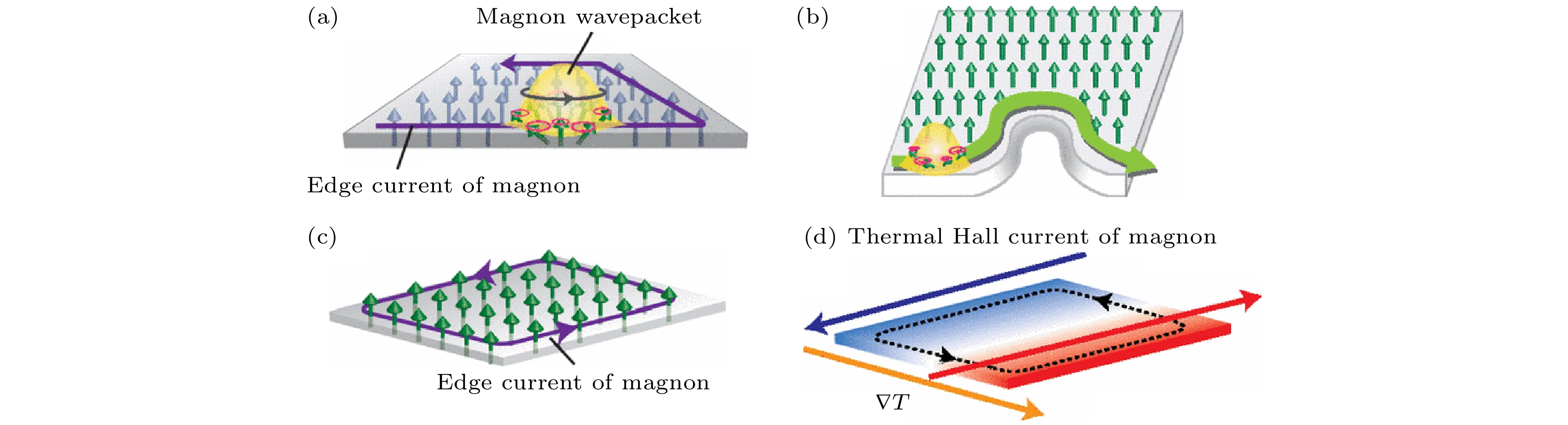
图 1 (a)磁子波包的自转和绕着系统边界的磁子流; (b)沿着边界传输且与边界形状无关的磁子流; (c)平衡态时的边界磁子流; (d)温度梯度导致的有限热霍尔磁子流[24]
Fig. 1. (a) Self-rotation of a magnon wave packet and a magnon edge current; (b) the magnon near the boundary proceeds along the boundary, irrespective of the edge shape; (c) magnon edge current in equilibrium; (d) under the temperature gradient, a finite thermal Hall current will appear[24]
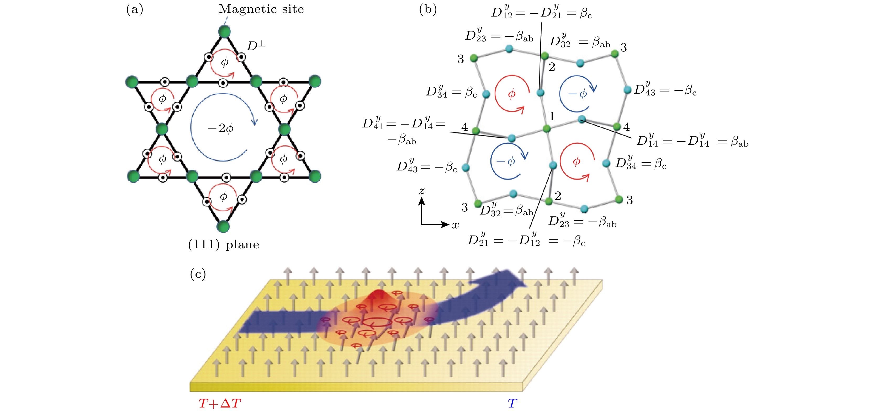
图 2 DM相互作用在烧绿石(111)平面中诱导的幅角$ \phi_i $分布(a)和在扭曲的钙钛矿的z-x平面中诱导的幅角分布(b)[30]; (c) 磁子的霍尔效应示意图[29]
Fig. 2. Spital distribution of $ \phi_i $ induced by DM interaction in the (111) plane of the pyrochlore lattice (a) and the z-x plane of the distorted perovskite structure (b)[30]; (c) schematic of magnon Hall effect[29]
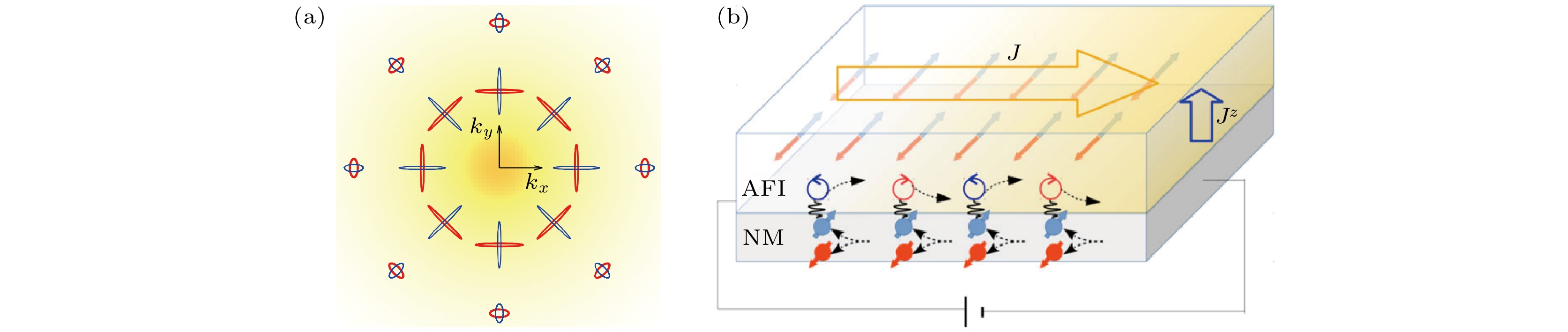

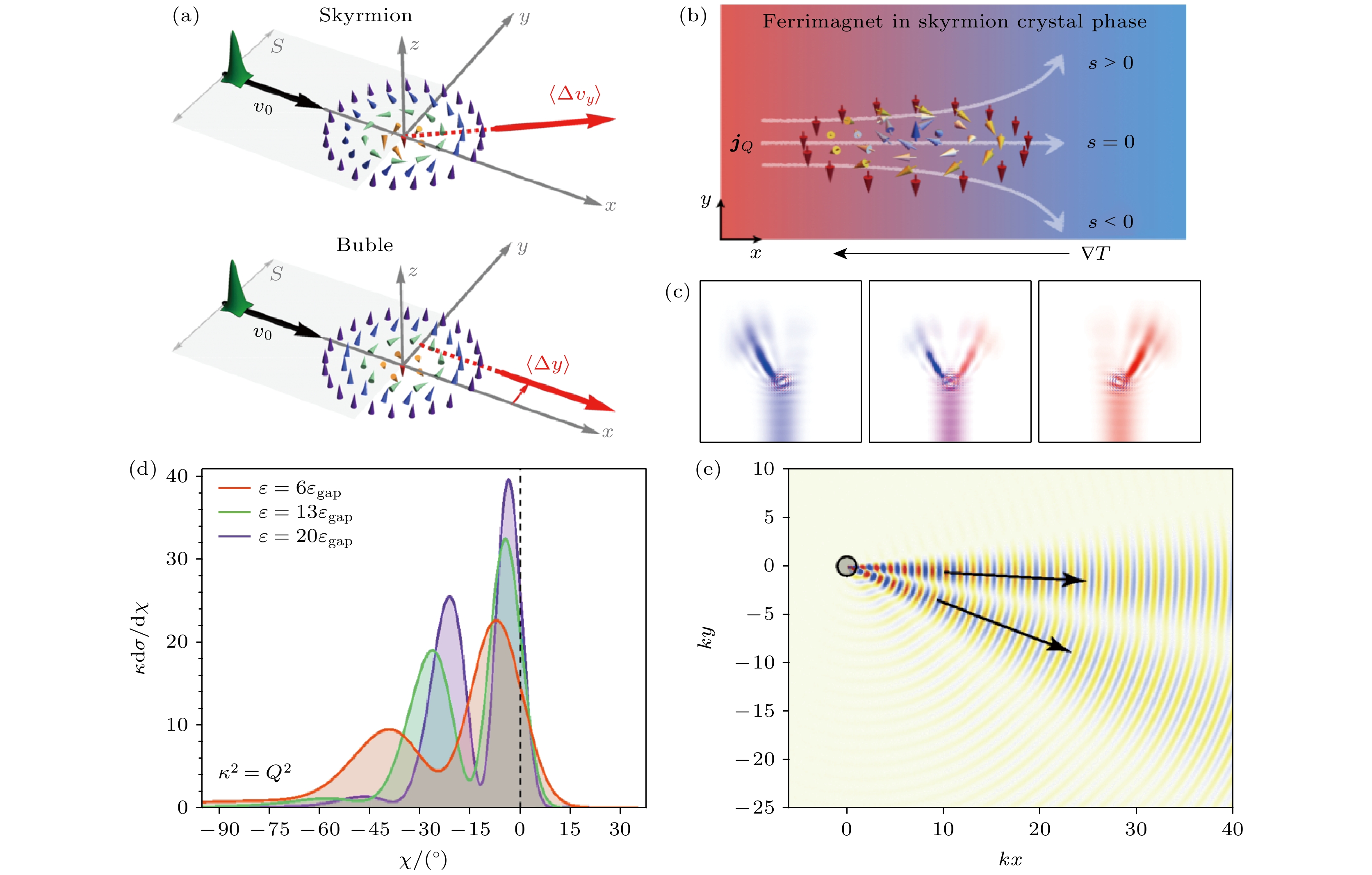
图 6 (a)磁子经过磁织构之后的斜散射和边跳跃行为[38]; 磁子经过(b)亚铁磁和(c)反铁磁斯格明子之后的偏转轨迹[42,43]; (d)散射理论计算得到的不同入射磁子能量下的微分散射截面, $ \varepsilon_{\rm gap} $为k = 0时的磁子能量[47]; (e)磁子的彩虹散射过程[47]
Fig. 6. (a) Skew scattering and side jump of spin wave across magnetic texture[38]; the trajectories of spin wave across (b) antiferromagnetic and (c) ferrimagnetic skyrmion[42,43]; (d) differential cross section evaluated from scattering theory for various energies, $ \varepsilon_{\rm gap} $ is the magnon gap[47] at k = 0; (e) the rainbow scattering process of magnons[47]

图 7 (a)由贝里曲率诱导的反常霍尔效应和贝里曲率偶极子诱导的非线性霍尔效应示意图[50]. (b)非线性磁子流和交换系数$ J_1 $的关系[51]. 磁子的(c)能带、(d)贝里曲率和(e)贝里曲率偶极子在动量空间的分布[51]
Fig. 7. (a) Schematics of the anomalous Hall effect induced by the finite Berry curvature and the nonlinear Hall effect induced by the finite Berry curvature dipoles in the entire space, respectively[50]. (b) Nonlinear magnon current as a function of exchange constant $ J_1 $[51]. Distribution of (c) the band structure, (d) berry curvature, and (e) berry curvature dipole of magnons in the momentum space[51]

图 9 (a)磁子非线性拓扑自旋霍尔效应示意图; (b)虚拟磁场B 和B'的空间分布以及对应磁子的运动轨迹(分别在B和B+B'作用下); (c)不同磁子模式的波函数的等值线分布; (d)线性非线性霍尔角和入射磁子频率$ \omega_{\mathrm{s}} $以及非线性阶数m的关系[59]
Fig. 9. (a) Schematic illustration of the nonlinear topological magnon spin Hall effect in magnon-AFM skyrmion scattering; (b) spatial distribution of dimensionless field B and B' as well as the corresponding spin wave trajectories in real space; (c) isoline maps for different magnon modes; (d) the Hall angle as a function of the incident magnon frequencie $ \omega_{\mathrm{s}} $ and mode index m[59]
-
[1] Žutić L, Fabian J, Sarma S D 2004 Rev. Mod. Phys. 76 323
Google Scholar
[2] Lenk B, Ulrichs H, Garbs F, Münzenberg M 2011 Phys. Rep. 507 107
Google Scholar
[3] Chumak A V, Vasyuchka V I, Serga A A, Hillebrands B 2015 Nat. Phys. 11 453
Google Scholar
[4] Yuan H Y, Cao Y, Kamra A, Duine R A, Yan P 2022 Phys. Rep. 965 1
Google Scholar
[5] Hall E H 1879 Am. J. Math. 2 287
Google Scholar
[6] Nagaosa N, Sinova J, Onoda S, MacDonald A H, Ong N P 2010 Rev. Mod. Phys. 82 1539
Google Scholar
[7] Jungwirth T, Niu Q, MacDonald A H 2002 Phys. Rev. Lett. 88 207208
Google Scholar
[8] Liang T, Lin J, Gibson Q, Kushwaha S, Liu M, Wang W, Xiong H, Sobota J A, Hashimoto M, Kirchmann P S, Shen Z, Cava R J, Ong N P 2018 Nat. Phys. 14 451
Google Scholar
[9] Tian Y, Ye L, Jin X 2009 Phys. Rev. Lett. 103 087206
Google Scholar
[10] Hirsch J E 1999 Phys. Rev. Lett. 83 1834
Google Scholar
[11] Sinova J, Culcer D, Niu Q, Sinitsyn N A, Jungwirth T, MacDonald A H 2004 Phys. Rev. Lett. 92 126603
Google Scholar
[12] Kato Y K, Myers R C, Niu Q, Gossard A C, Jawschalom D D 2004 Science 306 1910
Google Scholar
[13] Sinova J, Valenzuela S O, Wunderlich J, Back C H, Jungwirth T 2015 Rev. Mod. Phys. 87 1213
Google Scholar
[14] Neubauer A, Pfleiderer C, Binz B, Rosch A, Ritz R, Niklowitz P G, Böni P 2009 Phys. Rev. Lett. 102 186602
Google Scholar
[15] Yin G, Liu Y, Barlas Y, Zang J, Lake R K 2015 Phys. Rev. B 92 024411
Google Scholar
[16] Göbel B, Mook A, Henk J, Mertig I 2017 Phys. Rev. B 96 060406
Google Scholar
[17] Akosa C A, Tretiakov O A, Tatara G, Manchon A 2018 Phys. Rev. Lett. 121 097204
Google Scholar
[18] Berry M V 1984 Proc. R. Soc. A 392 45
[19] Skyrme T H R 1962 Nucl. Phys. 31 556
Google Scholar
[20] Mühlbauer S, Binz B, Jonietz F, Pfleiderer C, Rosch A, Neubauer A, Georgii R, Böni P 2009 Science 323 915
Google Scholar
[21] Yu X Z, Onose Y, Kanazawa N, Park J H, Han J H, Matsui Y, Nagaosa N, Tokura Y 2010 Nature 465 901
Google Scholar
[22] Heinze S, Bergmann K V, Menzel M, Brede J, Kubetzka A, Wiesendanger R, Bihlmayer G, Blügel S 2011 Nat. Phys. 7 713
Google Scholar
[23] Sundaram G, Niu Q 1999 Phys. Rev. B 59 14915
Google Scholar
[24] Matsumoto R, Murakami S 2011 Phys. Rev. Lett. 106 197202
Google Scholar
[25] Zhang L, Ren J, Wang J, Li B 2013 Phys. Rev. B 87 144101
Google Scholar
[26] Dzyaloshinsky I 1958 J. Phys. Chem. Solids 4 241
Google Scholar
[27] Moriya T 1960 Phys. Rev. 120 91
Google Scholar
[28] Katsura H, Nagaosa N, Lee P A 2010 Phys. Rev. Lett. 104 066403
Google Scholar
[29] Onose Y, Ideue T, Katsura H, Shiomi Y, Nagaosa N, Tokura Y 2010 Science 329 297
Google Scholar
[30] Ideue T, Onose Y, Katsura H, Shiomi Y, Ishiwata S, Nagaosa N, Tokura Y 2012 Phys. Rev. B 85 134411
Google Scholar
[31] Shen K 2020 Phys. Rev. Lett. 124 077201
Google Scholar
[32] Yu H, Xiao J, Schultheiss H 2021 Phys. Rep. 905 1
Google Scholar
[33] Li Z X, Cao Y, Yan P 2021 Phys. Rep. 915 1
Google Scholar
[34] Murakami S, Okamoto A 2017 J. Phys. Soc. Jpn. 86 011010
Google Scholar
[35] Serga A A, Chumak A V, Hillebrands B 2010 J. Phys. D: Appl. Phys. 43 264002
Google Scholar
[36] van Hoogdalem K A, Tserkovnyak Y, Loss D 2013 Phys. Rev. B 87 024402
Google Scholar
[37] Holstein T, Primakoff H 1940 Phys. Rev. 58 1098
Google Scholar
[38] Lan J, Xiao J 2021 Phys. Rev. B 103 054428
Google Scholar
[39] Lan J, Yu W, Xiao J 2021 Phys. Rev. B 103 214407
Google Scholar
[40] Thiele A A 1973 Phys. Rev. Lett. 30 230
Google Scholar
[41] Iwasaki J, Mochizuki M, Nagaosa N 2013 Nat. Commun. 4 1463
Google Scholar
[42] Daniels M W, Yu W, Cheng R, Xiao J, Xiao D 2019 Phys. Rev. B 99 224433
Google Scholar
[43] Kim S K, Nakata K, Loss D, Tserkovnyak Y 2019 Phys. Rev. Lett. 122 057204
Google Scholar
[44] Jin Z, Meng C Y, Liu T T, Chen D Y, Fan Z, Zeng M, Lu X B, Gao X S, Qin M H, Liu J M 2021 Phys. Rev. B 104 054419
Google Scholar
[45] Liu Y, Liu T T, Jin Z, Hou Z P, Chen D Y, Fan Z, Zeng M, Lu X B, Gao X S, Qin M H, Liu J M 2022 Phys. Rev. B 106 064424
Google Scholar
[46] Iwasaki J, Beekman A J, Nagaosa N 2014 Phys. Rev. B 89 064412
Google Scholar
[47] Schütte C, Garst M 2014 Phys. Rev. B 90 094423
Google Scholar
[48] Berry M V, Mount K E 1972 Rep. Progr. Phys. 35 315
Google Scholar
[49] Sodemann I, Fu L 2015 Phys. Rev. Lett. 115 216806
Google Scholar
[50] Ma Q, Xu S Y, Shen H, MacNeill D, Fatemi V, Chang T R, Valdivia A M M, Wu S, Du Z, Hsu C H, Fang S, Gibson Q D, Watanabe K, Taniguchi T, Cava R J, Kaxiras E, Lu H Z, Lin H, Fu L, Gedik N, Herrero P J 2019 Nature 565 337
Google Scholar
[51] Kondo H, Akagi Y 2022 Phys. Rev. Res. 4 013186
Google Scholar
[52] Schultheiss H, Janssens X, Kampen M V, Ciubotaru F, Hermsdoerfer S J, Obry B, Laraoui A, Serga A A, Lagae L, Slavin A N, Leven B, Hillebrands B 2009 Phys. Rev. Lett. 103 157202
Google Scholar
[53] Wang Z, Yuan H Y, Cao Y, Li Z, Duine R A, Yan P 2021 Phys. Rev. Lett. 127 037202
Google Scholar
[54] Wang Z, Yuan H Y, Cao Y, Yan P 2022 Phys. Rev. Lett. 129 107203
Google Scholar
[55] Schultheiss H, Vogt K, Hillebrands B 2012 Phys. Rev. B 86 054414
Google Scholar
[56] Tymchenko M, Gomez-Diaz J S, Lee J, Nookala N, Belkin M A, Alù A 2015 Phys. Rev. Lett. 115 207403
Google Scholar
[57] Li G, Chen S, Pholchai N, Reineke B, Wong P W H, Pun E Y B, Cheah K W, Zentgraf T, Zhang S 2015 Nat. Mater. 14 607
Google Scholar
[58] Li Y, Yesharim O, Hurvitz I, Karnieli A, Fu S, Porat G, Arie A 2020 Phys. Rev. A 101 033807
Google Scholar
[59] Jin Z, Yao X, Wang Z, Yuan H Y, Zeng Z, Wang W, Cao Y S, Yan P 2023 Phys. Rev. Lett. 131 166704
Google Scholar
[60] Zyuzin V A, Kovalev A A 2016 Phys. Rev. Lett. 117 217203
Google Scholar
[61] Xiao J, Bauer G E W, Uchida K, Saitoh E, Maekawa S 2000 Phys. Rev. B 81 214418
[62] Mook A, Plekhanov K, Klinovaja J, Loss D 2021 Phys. Rev. X 11 021061
[63] Zhang X, Zhang Y, Okamoto S, Xiao D 2019 Phys. Rev. Lett. 123 167202
Google Scholar
[64] Cao Y, Fatemi V, Demir A, Fang S, Tomarken S, Luo J, Sanchez-Yamagishi J, Watanabe K, Taniguchi T, Kaxiras E, Ashoori R, Jarillo-Herrero P 2018 Nature 556 80
[65] Cao Y, Fatemi V, Fang S, Watanabe K, Taniguchi T, Kaxiras E, Jarillo-Herrero P 2018 Nature 556 43
[66] Duan J, Jian Y, Gao Y, Peng H, Zhong J, Feng Q, Mao J, Yao Y 2022 Phys. Rev. Lett. 129 186801
Google Scholar
[67] Huang M, Wu Z, Zhang X, Feng X, Zhou Z, Wang S, Chen Y, Cheng C, Sun K, Meng Z Y, Wang N 2023 Phys. Rev. Lett. 131 066301
Google Scholar
[68] Wang H, Madami M, Chen J, et al. 2023 Phys. Rev. X 13 021016

 下载:
下载:
计量
- 文章访问数: 11507
- PDF下载量: 692
- 被引次数: 0
