


-
The wetting and spreading of droplets on solid walls are commonly seen in nature. The study of such a phenomenon can deepen our understanding of solid-liquid interaction and promote the development of relevant cutting-edge technological applications. In this work, the lattice Boltzmann method based on phase field theory is used to investigate the wetting and spreading of a compound droplet on a wedge. This method combines the finite-difference solution of the Cahn-Hilliard equations for ternary fluids to capture the interface dynamics and the lattice Boltzmann method for the hydrodynamics of the flow. Symmetric compound droplets with equal interfacial tensions on a wedge are considered first. Through theoretical analysis and numerical simulation, it is found that the wetted area on the wedge increases with the decrease of the contact angle of the wedge surface and the wedge apex angle. Depending on these two factors, the droplet may or may not split on the wedge. We also find that the droplet near the critical state predicted not to split by static equilibrium analysis could split during the spreading along the wall of the wedge under certain density and viscosity ratios. Based on the simulation results, a phase diagram of the droplet splitting state is generated with the density ratio and viscosity ratio as the coordinates. As the density ratio and kinematic viscosity ratio increase, the inertia effect becomes more prominent in the wetting and spreading process and the droplet is more likely to split. By comparing the phase diagrams in different initial conditions, it is found that under the same conditions, the compound droplet with an equilibrium initial state is less likely to split than that with an unequilibrium initial state, which is possibly because the initial total energy of the former is relatively small. Our study also shows that the kinematic viscosity ratio between the left half and the right half droplet may affect the results of droplet splitting. The increase of such a viscosity difference is conducive to the splitting of the compound droplet. Besides, asymmetric compound droplets with unequal interfacial tensions are also simulated, and it is found that the greater the wrapping degree between the left half and right half, the more difficult it is to separate the compound droplet.
-
Keywords:
- compound droplet /
- lattice Boltzmann method /
- wetting and spreading /
- split
[1] Latthe S S, Sutar R S, Kodag V S, et al. 2019 Prog. Org. Coat. 128 52
 Google Scholar
[2] Woerthmann B M, Totzauer L, Briesen H 2022 Powder Technol. 404 117443
Google Scholar
[3] Eres M H, Schwartz L W, Roy R V 2000 Phys. Fluids 12 1278
Google Scholar
[4] Dai Q W, Huang W, Wang X L, Khonsari M M 2021 Tribol. Int. 154 106749
Google Scholar
[5] Yang Y, Li X J, Zheng X, Chen Z Y, Zhou Q F, Chen Y 2018 Adv. Mater. 30 1704912
Google Scholar
[6] Young T 1805 Philos. Trans. R. Soc. London 95 65
[7] Sui T, Wang J D, Chen D R 2011 J. Colloid Interface Sci. 358 284
Google Scholar
[8] Li Y Q, Wu H A, Wang F C 2016 J. Phys. D Appl. Phys. 49 085304
Google Scholar
[9] Han Z Y, Duan L, Kang Q 2019 AIP Adv. 9 085203
Google Scholar
[10] Wang F, Schiller U D 2021 Soft Matter 17 5486
Google Scholar
[11] Herminghaus S, Brinkmann M, Seemann R 2008 Ann. Rev. Mater. Res. 38 101
Google Scholar
[12] Chang F M, Hong S J, Sheng Y J, Tsao H K 2010 J. Phys. Chem. C 114 1615
Google Scholar
[13] Zhou L M, Yang S M, Quan N N, et al. 2021 ACS Appl. Mater. Interfaces 13 55726
Google Scholar
[14] Ma B J, Shan L, Dogruoz B, Agonafer D 2019 Langmuir 35 12264
Google Scholar
[15] Courbin L, Bird J C, Reyssat M, Stone H A 2009 J. Phys. Condes. Matter 21 464127
Google Scholar
[16] Frank X, Perre P 2012 Phys. Fluids 24 042101
Google Scholar
[17] Lee Y, Matsushima N, Yada S, Nita S, Kodama T, Amberg G, Shiomi J 2019 Sci. Rep. 9 7787
Google Scholar
[18] Ben Said M, Selzer M, Nestler B, Braun D, Greiner C, Garcke H 2014 Langmuir 30 4033
Google Scholar
[19] Weyer F, Ben Said M, Hotzer J, Berghoff M, Dreesen L, Nestler B, Vandewalle N 2015 Langmuir 31 7799
Google Scholar
[20] Zhang C Y, Ding H, Gao P, Wu Y L 2016 J. Comput. Phys. 309 37
Google Scholar
[21] He Q, Li Y J, Huang W F, Hu Y, Wang Y M 2020 Phys. Rev. E 101 033307
Google Scholar
[22] Li S, Lu Y, Jiang F, Liu H H 2021 Phys. Rev. E 104 015310
Google Scholar
[23] Huang J J 2021 Phys. Fluids 33 072105
Google Scholar
[24] Chen S Y, Doolen G D 1998 Annu. Rev. Fluid Mech. 30 329
Google Scholar
[25] Jacqmin D 1999 J. Comput. Phys. 155 96
Google Scholar
[26] Huang J J, Wu J, Huang H B 2018 Eur. Phys. J. E 41 1
Google Scholar
[27] Liang H, Chai Z H, Shi B C, Guo Z L, Zhang T 2014 Phys. Rev. E 90 063311
Google Scholar
[28] Lee T 2009 Comput. Math. Appl. 58 987
Google Scholar
[29] Bouzidi M, Firdaouss M, Lallemand P 2001 Phys. Fluids 13 3452
Google Scholar
[30] Lallemand P, Luo L S 2000 Phys. Rev. E 61 6546
Google Scholar
[31] Guo Z L, Shi B C, Zheng C G 2011 Philos. Trans. R. Soc. A Math. Phys. Eng. Sci. 369 2283
Google Scholar
[32] Carlson A, Do-Quang M, Amberg G 2011 J. Fluid Mech. 682 213
Google Scholar
-
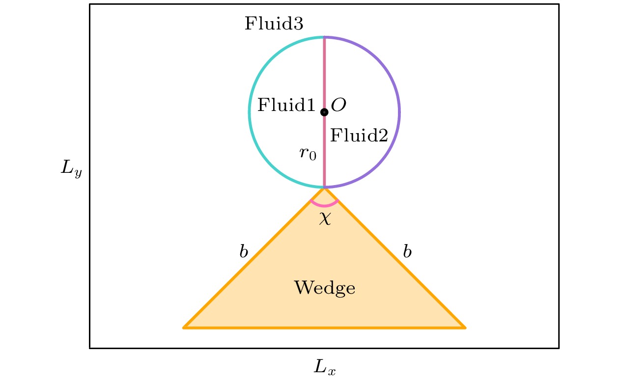
图 1 物理模型图示
Figure 1. Physical model illustration.
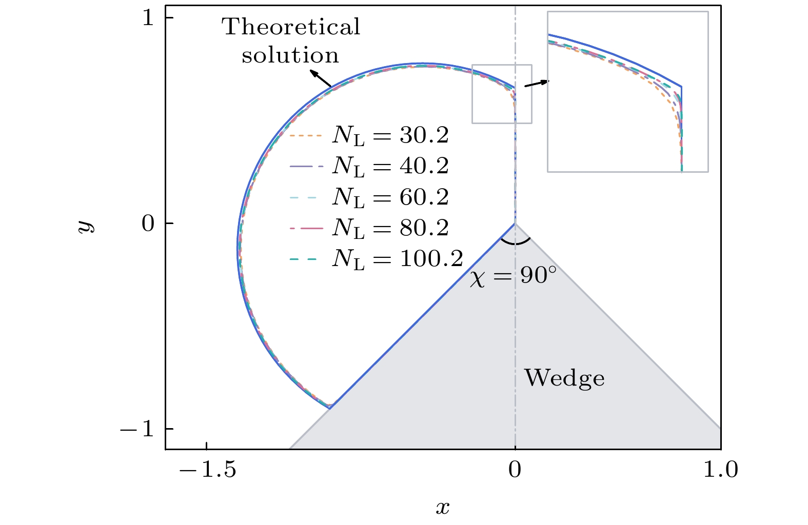
图 2 不同网格密度下液滴的平衡形态
Figure 2. Equilibrium morphology of the droplet at different mesh densities.

图 3 不同网格密度下液滴接触线位置的演化 (a)
$ {r_{{\rho _{13}}}} = $ $ {r_{{\nu _{13}}}} = 1 $ ; (b)$ {r_{{\rho _{13}}}} = {r_{{\nu _{13}}}} = 10 $ Figure 3. Evolution of the contact line position of droplet under the different mesh densities: (a)
$ {r_{{\rho _{13}}}} = {r_{{\nu _{13}}}} = 1 $ ;(b)$ {r_{{\rho _{13}}}} = $ $ {r_{{\nu _{13}}}} = 10 $ .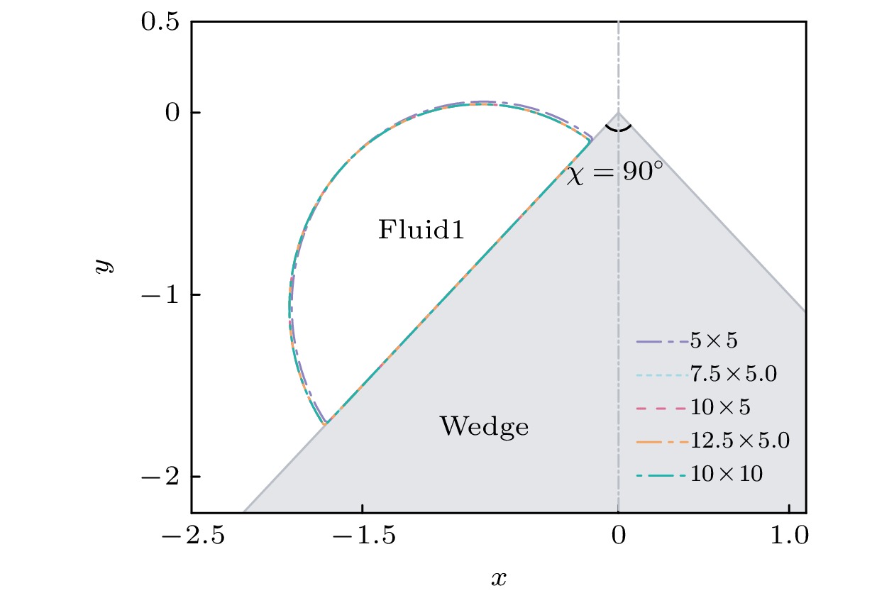
图 4 不同计算域
$ {L_x} \times {L_y} $ 下液滴的平衡形态Figure 4. Equilibrium morphology of droplets in different computational domains of
$ {L_x} \times {L_y} $ .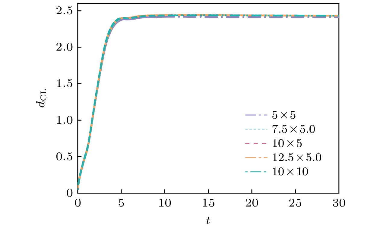
图 5 不同计算域
$ {L_x} \times {L_y} $ 下液滴接触线位置的演化Figure 5. Evolution of the contact line position of the droplet in different computational domains of
$ {L_x} \times {L_y} $ .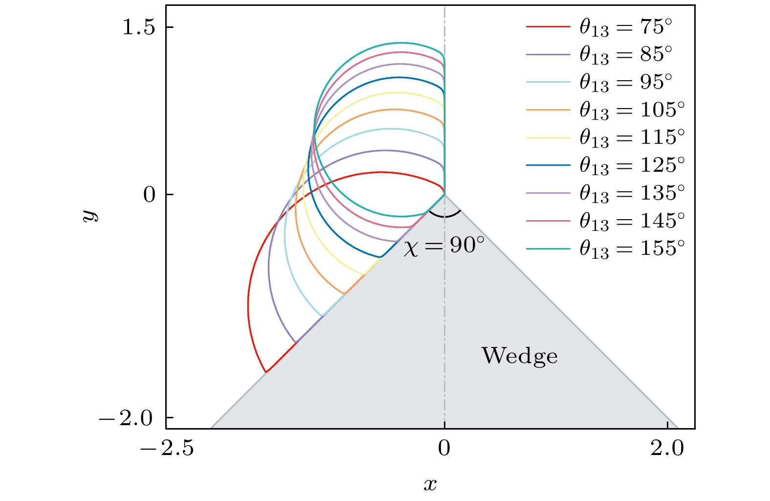
图 6 不同接触角下的液滴平衡形态
Figure 6. Equilibrium morphology of droplets at different contact angles.

图 7 h随接触角的变化曲线
Figure 7. Variation of h with the contact angle.
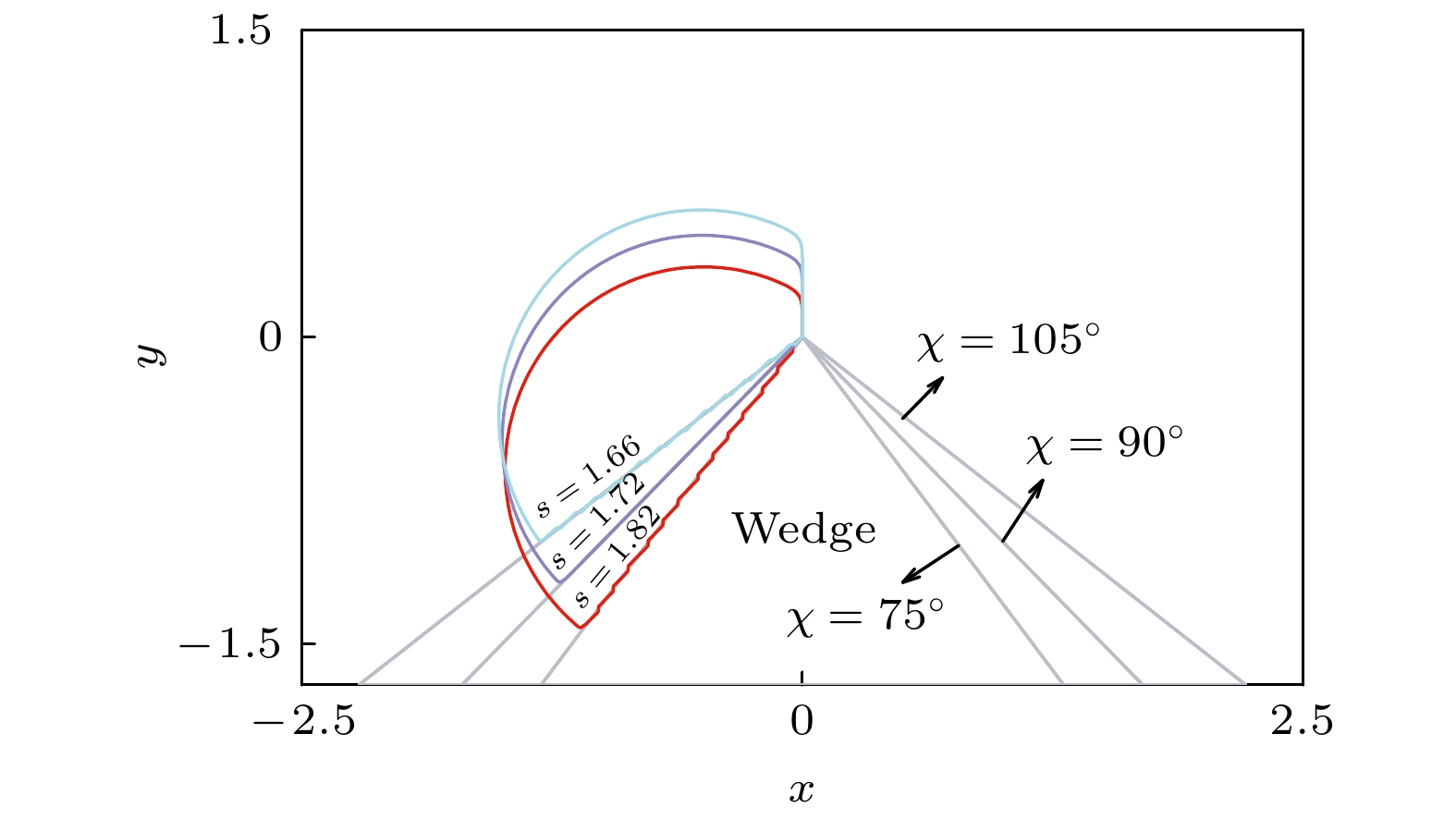
图 8 不同顶角楔形体上液滴的平衡形态
Figure 8. Equilibrium morphology of droplets on wedges with different vertex angles.
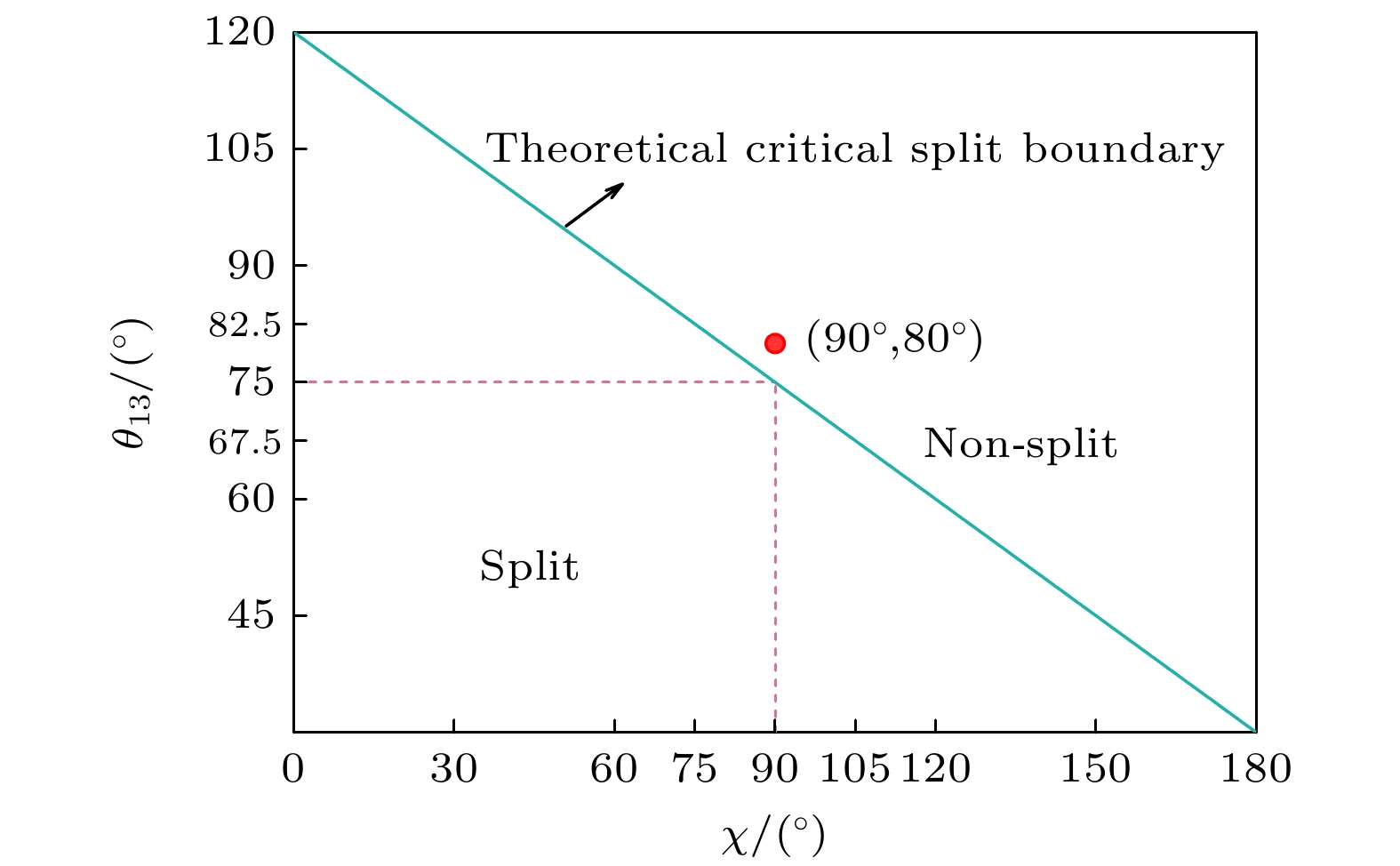
图 9 液滴分裂/不分裂理论临界界线
Figure 9. Theoretical critical boundary of droplet splitting/non-splitting state.
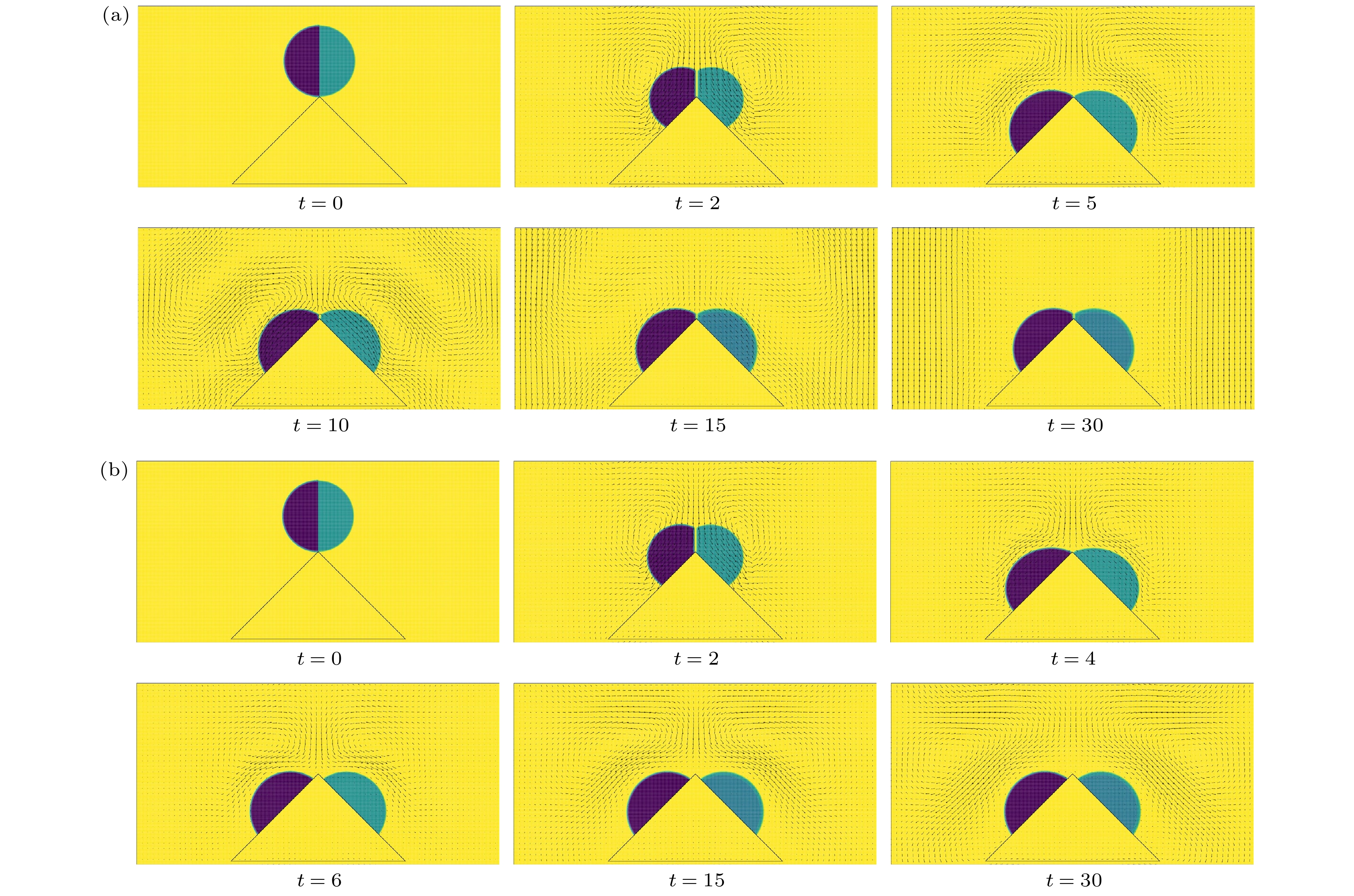
图 10 初始状态为非平衡态Janus状液滴的润湿铺展过程及速度场分布 (a)
$ {r_{{\rho _{13}}}} = 50 $ ,$ {r_{{\nu _{13}}}} = 1 $ ; (b)$ {r_{{\rho _{13}}}} = 50 $ ,$ {r_{{\nu _{13}}}} = 5 $ Figure 10. Wetting and spreading process and velocity field distribution of Janus-like droplet with non-equilibrium initial state: (a)
$ {r_{{\rho _{13}}}} = 50 $ ,$ {r_{{\nu _{13}}}} = 1 $ ; (b)$ {r_{{\rho _{13}}}} = 50 $ ,$ {r_{{\nu _{13}}}} = 5 $ .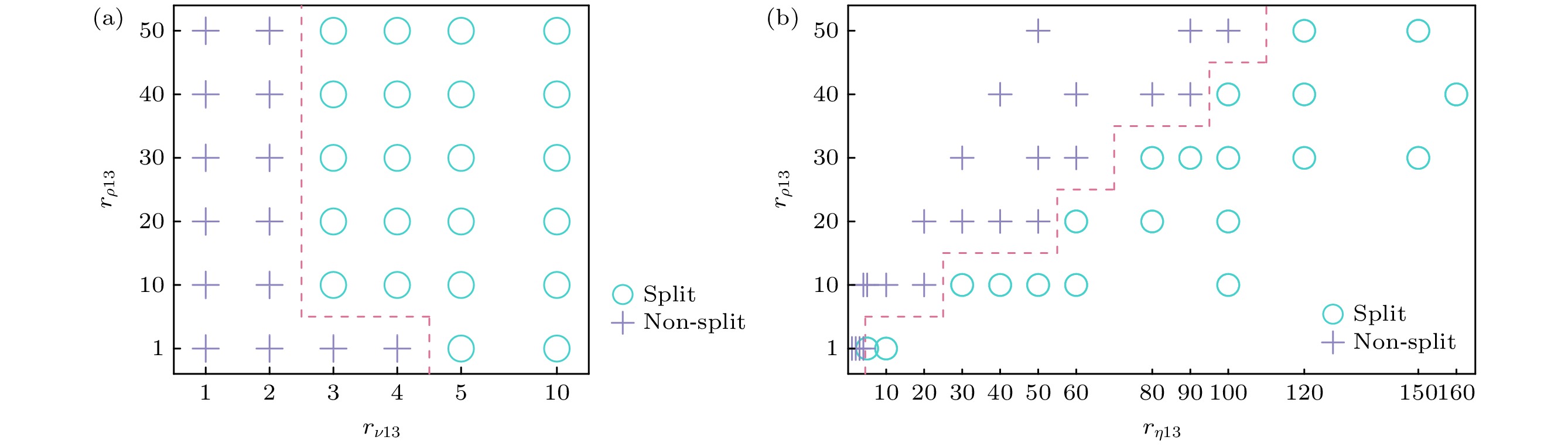
图 11 初始状态为非平衡态Janus状液滴的润湿分裂状态相图 (a) rv13 - rρ13; (b) rη13 - rρ13
Figure 11. Split/Non-split phase diagram of Janus-like droplets with non-equilibrium initial state: (a) rv13 vs. rρ13; (b) rη13 vs. rρ13.

图 12 初始状态为非平衡态时系统动能最大值随运动黏度比的变化曲线
Figure 12. Variation of the maximum kinetic energy of the system with the kinematic viscosity ratio under the non-equilibrium initial state.
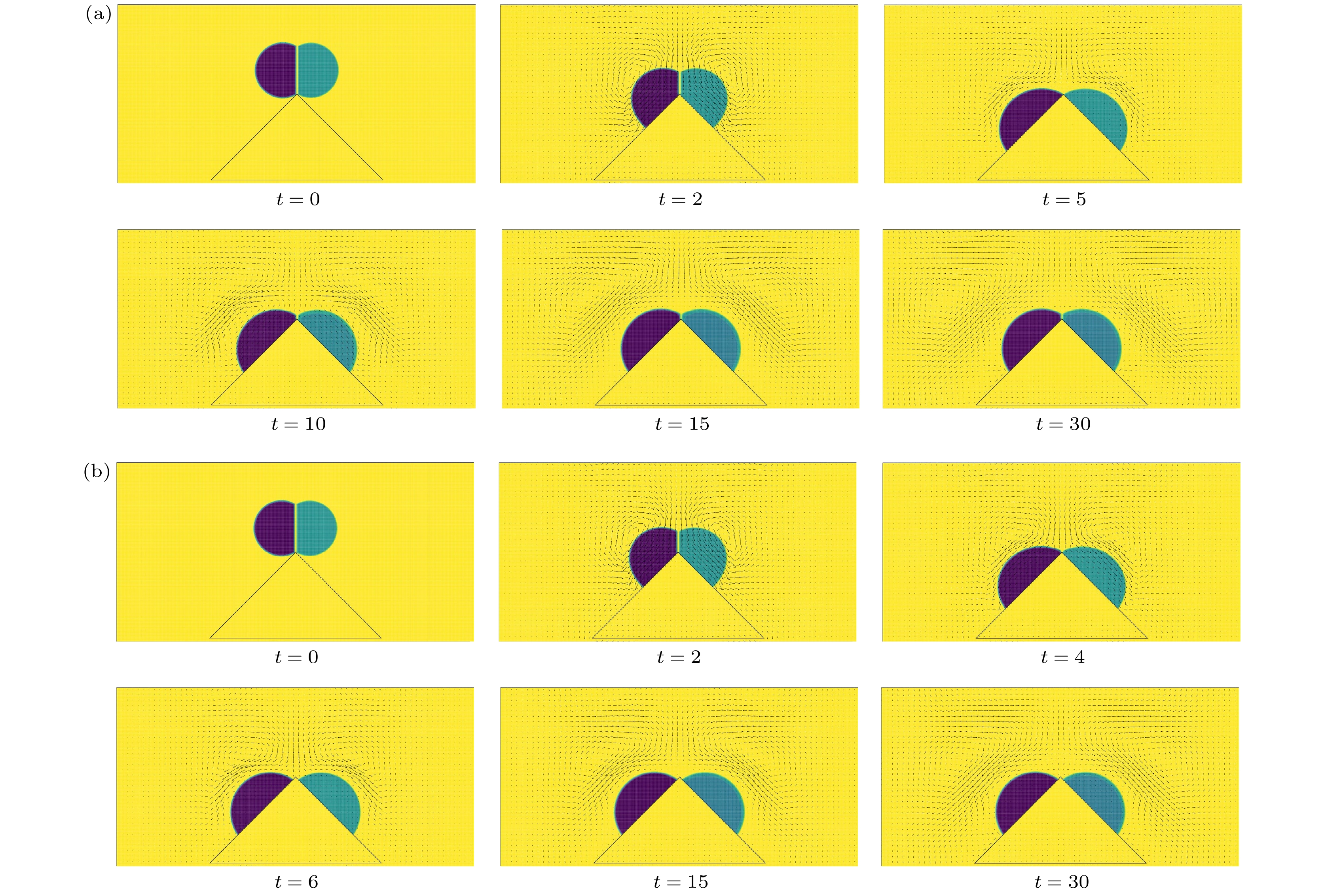
图 13 初始状态为平衡态复合液滴的润湿铺展过程及速度场分布 (a)
$ {r_{{\rho _{13}}}} = 50 $ ,$ {r_{{\nu _{13}}}} = 5 $ ; (b)$ {r_{{\rho _{13}}}} = 50 $ ,$ {r_{{\nu _{13}}}} = 10 $ Figure 13. Wetting and spreading process and velocity field distribution of compound droplet with equilibrium initial state: (a)
$ {r_{{\rho _{13}}}} = 50 $ ,$ {r_{{\nu _{13}}}} = 5 $ ; (b)$ {r_{{\rho _{13}}}} = 50 $ ,$ {r_{{\nu _{13}}}} = 10 $ .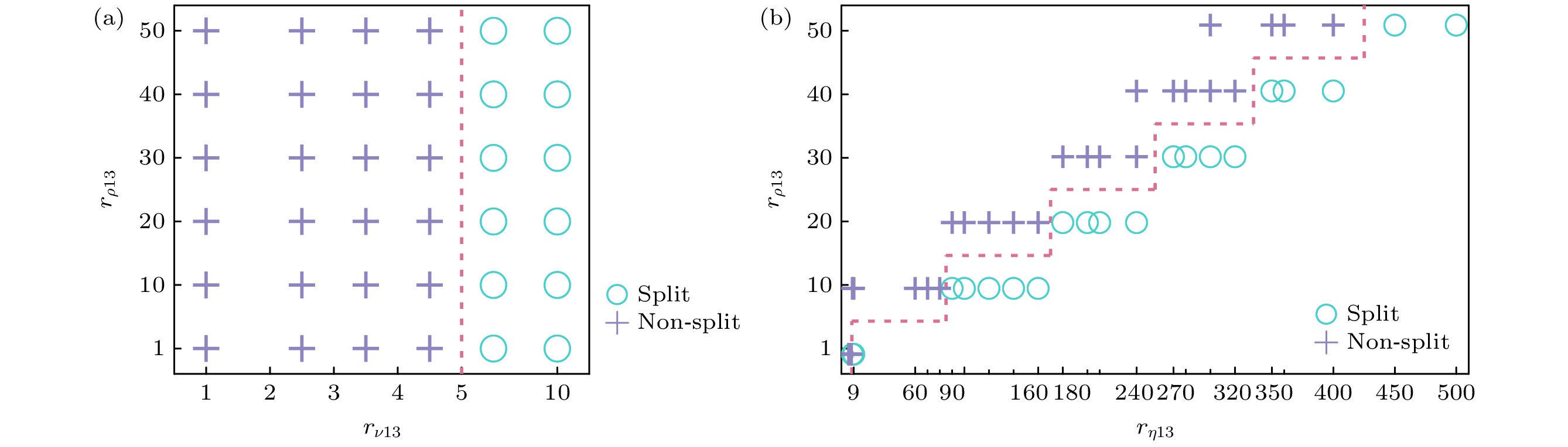
图 14 初始状态为平衡态复合液滴的润湿分裂状态相图 (a) rv13 - rρ13; (b) rη13 - rρ13
Figure 14. Split/non-split phase diagram of compound droplets with equilibrium initial state: (a) rv13 vs. rρ13; (b) rη13 vs. rρ13

图 15 左右侧液滴接触线位置的演化
Figure 15. Evolution of the position of the left and right droplet contact lines.
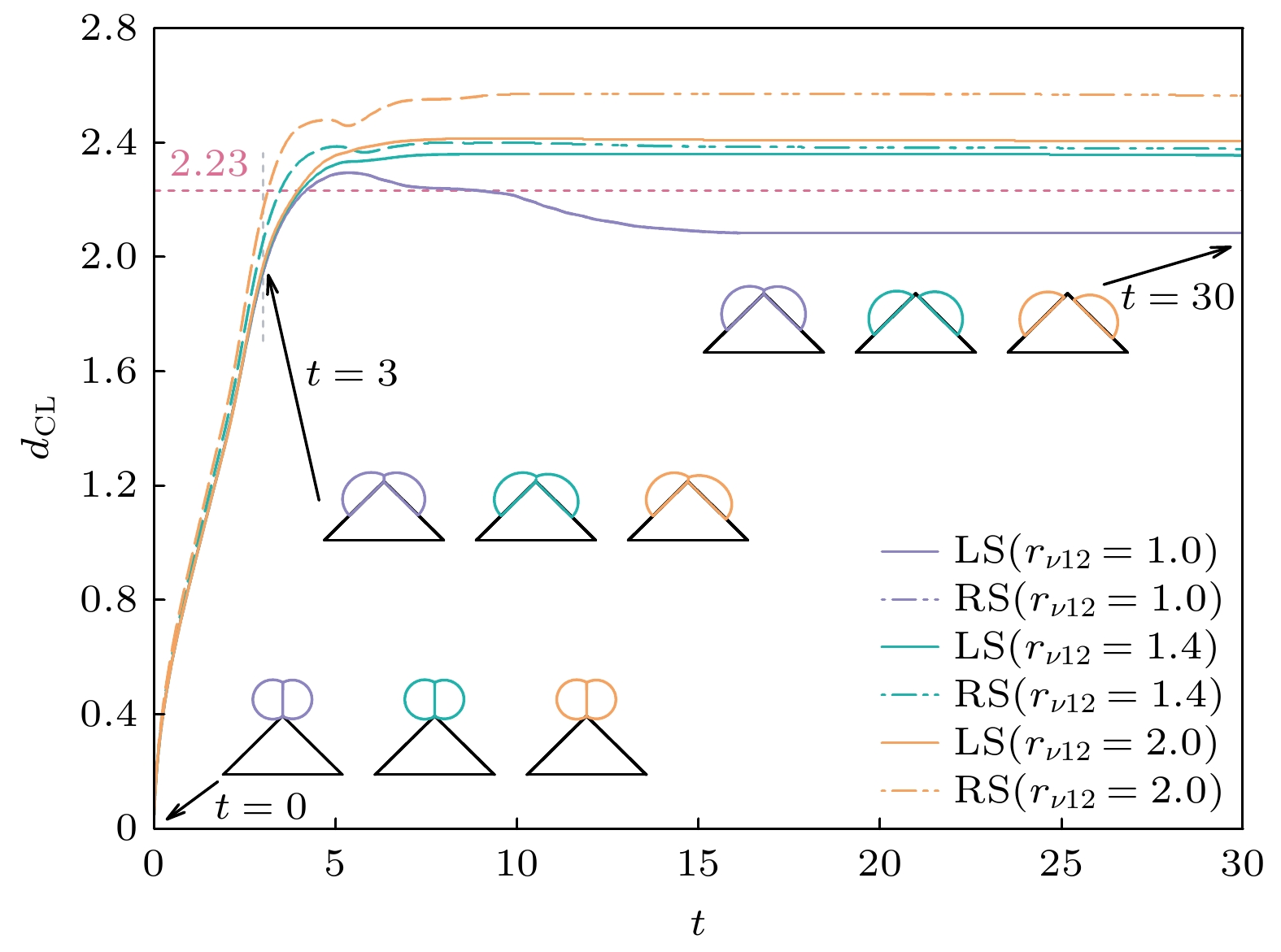
图 16 左右侧液滴接触线位置的演化
Figure 16. Evolution of the position of the left and right droplet contact lines.
-
[1] Latthe S S, Sutar R S, Kodag V S, et al. 2019 Prog. Org. Coat. 128 52
Google Scholar
[2] Woerthmann B M, Totzauer L, Briesen H 2022 Powder Technol. 404 117443
Google Scholar
[3] Eres M H, Schwartz L W, Roy R V 2000 Phys. Fluids 12 1278
Google Scholar
[4] Dai Q W, Huang W, Wang X L, Khonsari M M 2021 Tribol. Int. 154 106749
Google Scholar
[5] Yang Y, Li X J, Zheng X, Chen Z Y, Zhou Q F, Chen Y 2018 Adv. Mater. 30 1704912
Google Scholar
[6] Young T 1805 Philos. Trans. R. Soc. London 95 65
[7] Sui T, Wang J D, Chen D R 2011 J. Colloid Interface Sci. 358 284
Google Scholar
[8] Li Y Q, Wu H A, Wang F C 2016 J. Phys. D Appl. Phys. 49 085304
Google Scholar
[9] Han Z Y, Duan L, Kang Q 2019 AIP Adv. 9 085203
Google Scholar
[10] Wang F, Schiller U D 2021 Soft Matter 17 5486
Google Scholar
[11] Herminghaus S, Brinkmann M, Seemann R 2008 Ann. Rev. Mater. Res. 38 101
Google Scholar
[12] Chang F M, Hong S J, Sheng Y J, Tsao H K 2010 J. Phys. Chem. C 114 1615
Google Scholar
[13] Zhou L M, Yang S M, Quan N N, et al. 2021 ACS Appl. Mater. Interfaces 13 55726
Google Scholar
[14] Ma B J, Shan L, Dogruoz B, Agonafer D 2019 Langmuir 35 12264
Google Scholar
[15] Courbin L, Bird J C, Reyssat M, Stone H A 2009 J. Phys. Condes. Matter 21 464127
Google Scholar
[16] Frank X, Perre P 2012 Phys. Fluids 24 042101
Google Scholar
[17] Lee Y, Matsushima N, Yada S, Nita S, Kodama T, Amberg G, Shiomi J 2019 Sci. Rep. 9 7787
Google Scholar
[18] Ben Said M, Selzer M, Nestler B, Braun D, Greiner C, Garcke H 2014 Langmuir 30 4033
Google Scholar
[19] Weyer F, Ben Said M, Hotzer J, Berghoff M, Dreesen L, Nestler B, Vandewalle N 2015 Langmuir 31 7799
Google Scholar
[20] Zhang C Y, Ding H, Gao P, Wu Y L 2016 J. Comput. Phys. 309 37
Google Scholar
[21] He Q, Li Y J, Huang W F, Hu Y, Wang Y M 2020 Phys. Rev. E 101 033307
Google Scholar
[22] Li S, Lu Y, Jiang F, Liu H H 2021 Phys. Rev. E 104 015310
Google Scholar
[23] Huang J J 2021 Phys. Fluids 33 072105
Google Scholar
[24] Chen S Y, Doolen G D 1998 Annu. Rev. Fluid Mech. 30 329
Google Scholar
[25] Jacqmin D 1999 J. Comput. Phys. 155 96
Google Scholar
[26] Huang J J, Wu J, Huang H B 2018 Eur. Phys. J. E 41 1
Google Scholar
[27] Liang H, Chai Z H, Shi B C, Guo Z L, Zhang T 2014 Phys. Rev. E 90 063311
Google Scholar
[28] Lee T 2009 Comput. Math. Appl. 58 987
Google Scholar
[29] Bouzidi M, Firdaouss M, Lallemand P 2001 Phys. Fluids 13 3452
Google Scholar
[30] Lallemand P, Luo L S 2000 Phys. Rev. E 61 6546
Google Scholar
[31] Guo Z L, Shi B C, Zheng C G 2011 Philos. Trans. R. Soc. A Math. Phys. Eng. Sci. 369 2283
Google Scholar
[32] Carlson A, Do-Quang M, Amberg G 2011 J. Fluid Mech. 682 213
Google Scholar
-
 2-20221472补充材料+.pdf


 DownLoad:


Catalog
Metrics
- Abstract views: 5838
- PDF Downloads: 74
- Cited By: 0
