-
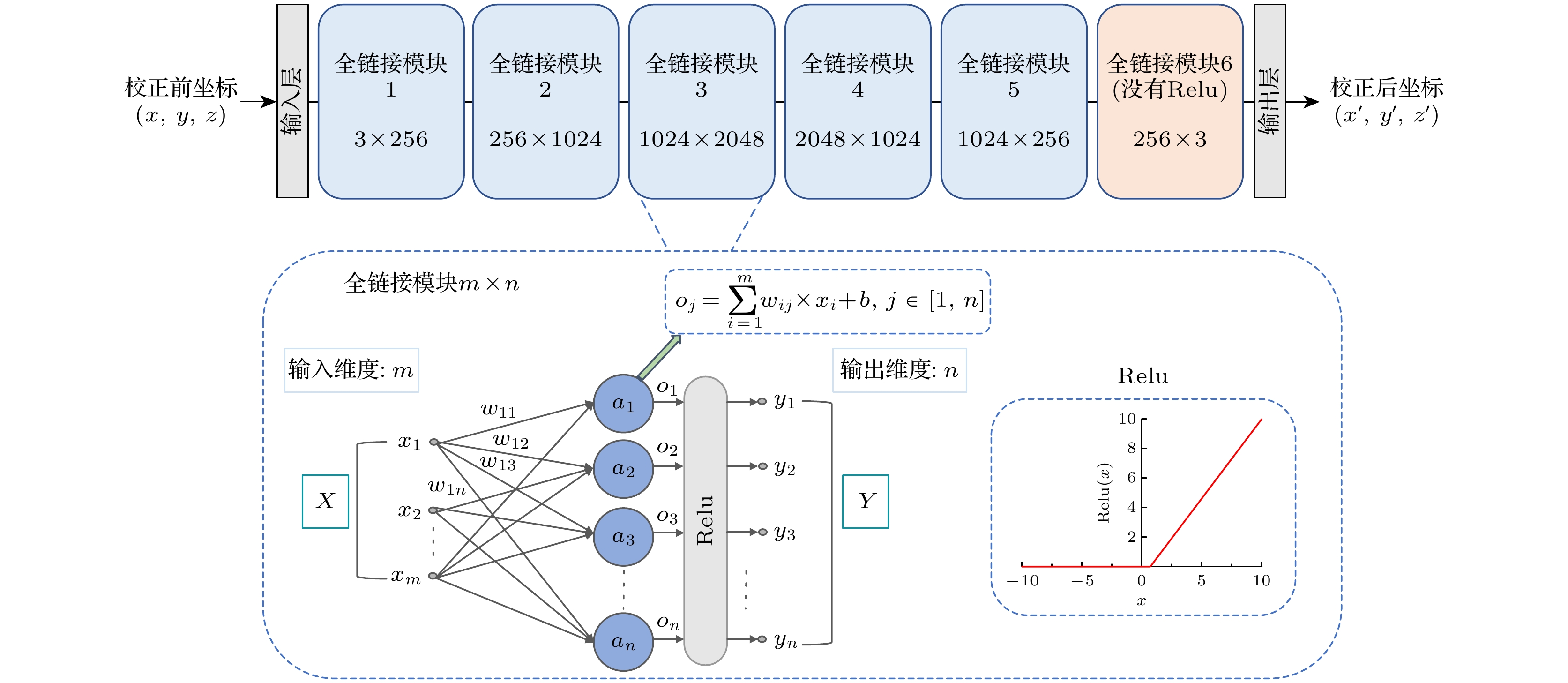
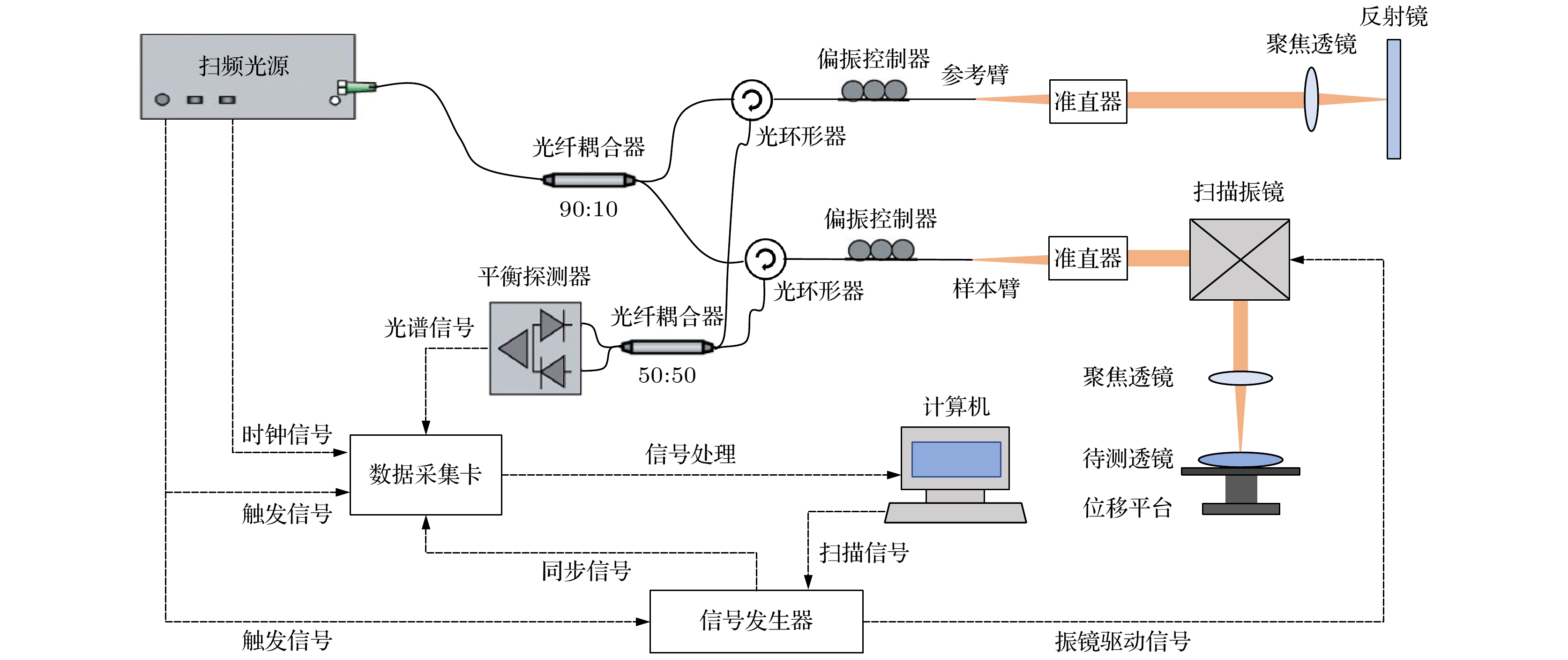
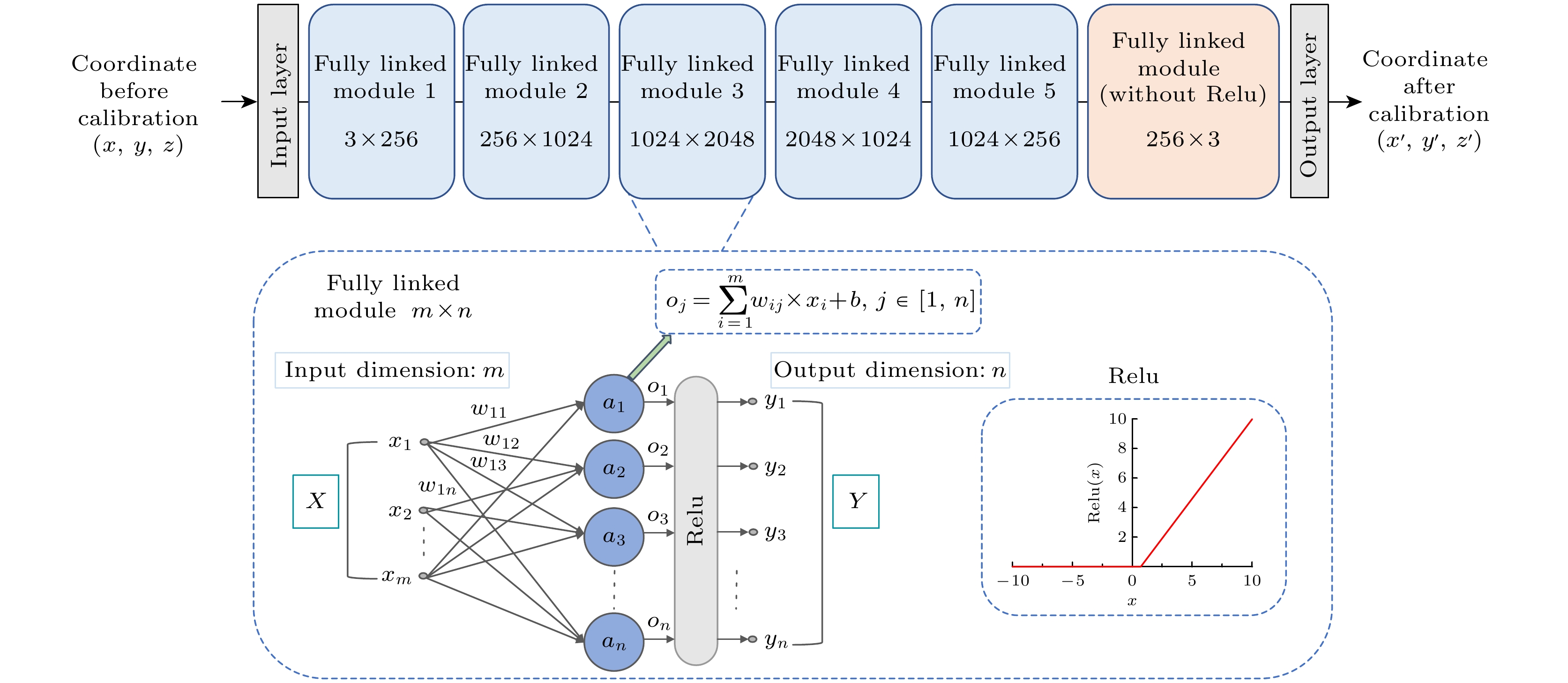
光学相干断层扫描(optical coherence tomography, OCT)成像中不可避免的畸变常常导致成像空间与真实空间之间的不匹配, 影响测量的准确性. 为解决该问题, 本研究提出了一种基于机器学习的OCT图像畸变校正方法. 首先, 将带有均匀分布圆孔阵列的校准板依次在不同标记平面进行成像. 选取坐标与所有成像平面的平均坐标偏差最小的点作为参考标记点. 然后, 利用数学模型重构参考平面上所有标记点的坐标, 从而建立校准板成像空间与真实物理空间之间的映射关系. 采用多层感知机来学习这种映射关系. 利用训练完成的模型推导整个空间点的分布规律, 从而实现透镜OCT图像的畸变校正, 并求出透镜中心厚度与曲率半径. 校正后透镜曲率半径精度达到10 μm, 误差在1%以内. 中心厚度精度可达3 μm, 相对误差为0.3%.The inevitable distortions in optical coherence tomography (OCT) imaging often lead to mismatches between the imaging space and the real space, significantly affecting measurement accuracy. To address this issue, this study proposes a machine learning-based OCT image distortion correction method. A calibration plate with uniformly distributed circular hole arrays is sequentially imaged at different marked planes. The point showing minimal deviation between its coordinates and the mean coordinates in all imaging planes is selected as a reference marker. A mathematical model is then used to reconstruct all marker point coordinates in the reference plane, establishing a mapping relationship between the imaging space of calibration plate and the real physical space. A multilayer perceptron (MLP) is employed to learn this mapping relationship. The network architecture consists of multiple fully-connected modules, each with a linear layer and an activation function besides the output layer. The optimal model is selected based on validation set performance, and then used to analyze the spatial distribution of points. Using a swept-source OCT system, lens images are acquired and corrected through the trained model to obtain the anterior surface point cloud. Combined with ray tracing reconstruction of the posterior surface, the lens curvature radius and central thickness are calculated. The experimental results show that after correction, the lens curvature radius is measured with an accuracy of 10 μm (error < 1%), while the central thickness is determined, with an accuracy of 3 μm (relative error: 0.3%). This method shows high accuracy and reliability, providing an effective solution for improving OCT measurement accuracy.
[1] Huang D, Swanson E A, Lin C P, Schuman J S, Stinson W G, Chang W, Hee M R, Flotte T, Gregory K, Puliafito C A, Fujimoto J G 1991 Science 254 1178
 Google Scholar
[2] Tomlins P H, Wang R K 2005 J. Phys. D Appl. Phys. 38 2519
 Google Scholar
[3] 丁宇韬, 张君, 郭遥, 陈昊 2024 激光与光电子学进展 61 247
Ding Y T, Zhang J, Guo Y, Chen H 2024 Laser Optoelectron. Prog. 61 247
[4] Volker W, Andrew R, Sunita R, Joseph I 2002 Opt. Express 10 397
 Google Scholar
[5] Diaz J, Rahlves M, Majdani O, Reithmeier E, Ortmaier T 2012 Optical Metrology and Inspection for Industrial Applications II Beijing, China, November 5–7, 2012 p8563J
[6] Yao J, Anderson A, Rolland J P 2018 Opt. Express 26 10242
 Google Scholar
[7] 江祥奎, 范永青, 王婉 2014 计算机科学与探索 8 1254
 Google Scholar
Jiang X Q, Fan Y Q, Wang W 2014 J. Front. Comput. Sci. Technol 8 1254
 Google Scholar
[8] 齐召帅, 王昭, 黄军辉, 薛琦, 高建民 2016 光子学报 45 87
Qi Z S, Wang Z, Huang J H, Xue Q, Gao J M 2016 Acta Photonica Sin. 45 87
[9] Lecun Y, Bottou L, Bengio Y, Haffner P 1998 Proc. IEEE 86 2278
 Google Scholar
[10] Li X Y, Zhang B, Sander P V, Liao J 2019 2019 IEEE/CVF Conference on Computer Vision and Pattern Recognition (CVPR) Long Beach, CA, USA, June 15–20, 2019 p4850
[11] Yang S R, Lin C Y, Liao K, Zhang C J, Zhao Y 2021 2021 IEEE/CVF Conference on Computer Vision and Pattern Recognition (CVPR) Nashville, TN, USA, June 20–25, 2021 p6344
[12] 徐启伟, 王佩佩, 曾镇佳, 黄泽斌, 周新星, 刘俊敏, 李瑛, 陈书青, 范滇元 2020 物理学报 69 014209
 Google Scholar
Xu Q W, Wang P P, Zeng Z J, Huang Z B, Zhou X X, Liu J M, Li Y, Chen S Q, Fan D Y 2020 Acta Phys. Sin. 69 014209
 Google Scholar
[13] 周静, 张晓芳, 赵延庚 2021 物理学报 70 054201
 Google Scholar
Zhou J, Zhang X F, Zhao Y G 2021 Acta Phys. Sin. 70 054201
 Google Scholar
[14] Shukla S, Vishwakarma C, Sah A N, Ahirwar S, Pandey K, Pradhan A 2023 Appl. Opt. 62 6826
 Google Scholar
[15] Breiman L, 2001 Mach. Learn. 45 5
 Google Scholar
[16] 谢探阳, 李玉梅, 张涛, 高天亮, 石玉超 2023 组合机床与自动化加工技术 2 37
Xie T Y, Li Y M, Zhang T, Gao T L, Shi Y C 2023 Mod. Mach. Tool Autom. Manuf. Tech. 2 37
[17] Kato D, Maeda N, Hirogaki T, Aoyama E, Takahashi K 2021 2021 21st International Conference on Control, Automation and Systems Jeju, Korea, October 12–15, 2021 p607
[18] Werbos P J 1981 System Modeling and Optimization Berlin, Germany, July 20–24, 1981 p762
[19] Rumelhart D E, Hinton G E, Williams R J 1986 Nature 323 533
 Google Scholar
[20] 杨沅松, 王晰, 任明俊 2023 光学学报 43 200
Yang Y S, Wang X, Ren M J 2023 Acta Opt. Sin. 43 200
[21] Singarimbun R N, Nababan E B, Sitompul O S 2019 2019 International Conference of Computer Science and Information Technology (ICoSNIKOM) Medan, Indonesia, November 28–29, 2019 p1
[22] Cotter A, Shamir O, Srebro N, Sridharan K 2011 Advances in Neural Information Processing Systems Granada, Spain, December 12–15, 2011 p1647
[23] Fitzgibbon A, Pilu M, Fisher R B 1999 IEEE Trans. Pattern Anal. Mach. Intell. 21 476
 Google Scholar
-
图 4 成像空间中标记点及其坐标的确定流程 (a)标定板横断面图; (b) “圆孔”区域与背景区域的划分; (c)分割模板; (d)基于“圆孔”区域质心的标记点分布图
Fig. 4. Process for the determination of marker points and their coordinates in the imaging space: (a) Cross-sectional view of the calibration plate; (b) division of the “circular hole” regions from the background; (c) segmentation template; (d) distribution map of marker points by centroids of the “circular hole” regions.
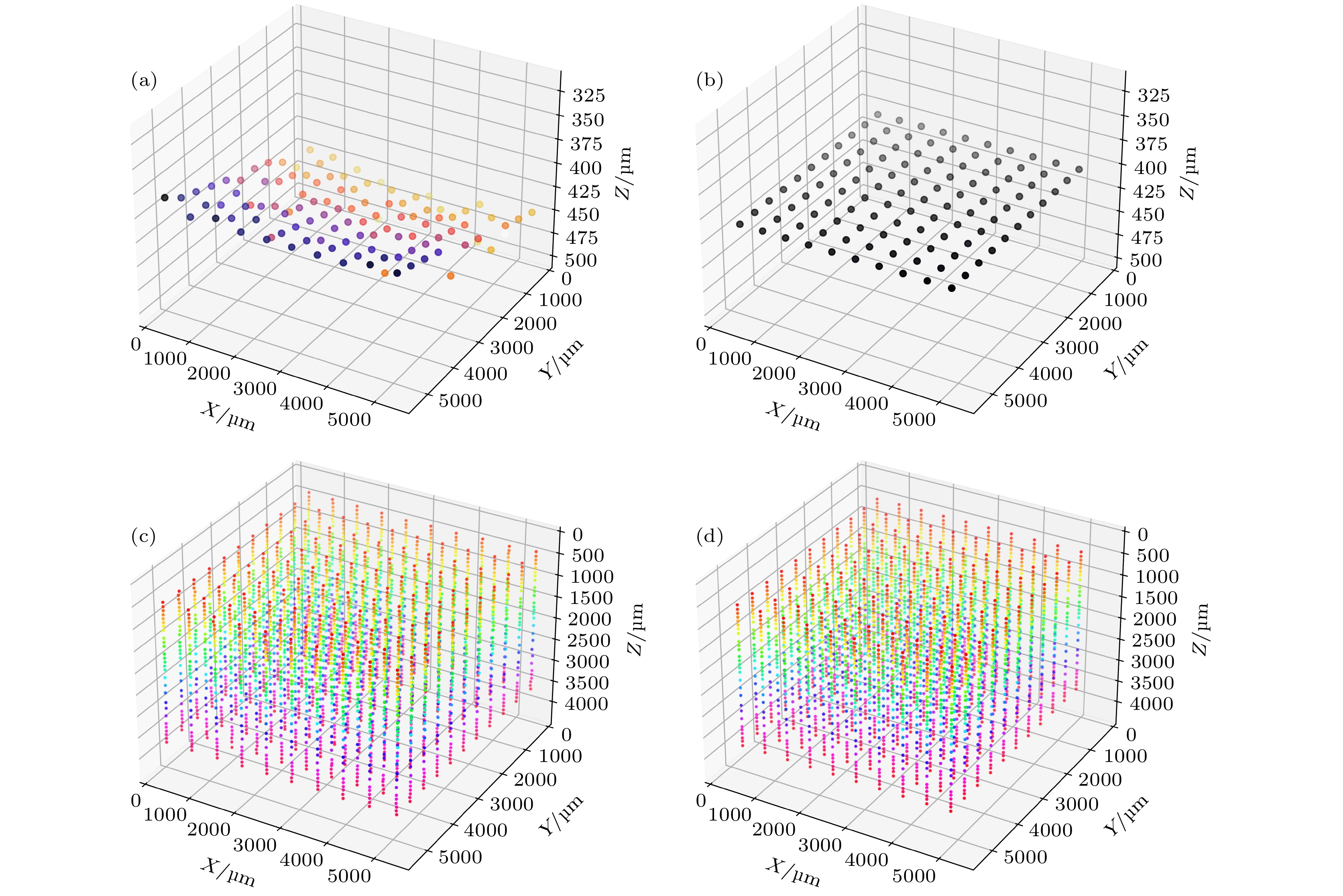
图 5 标记点点云分布 (a)成像空间单层点云分布; (b)真实空间单层点云分布; (c)成像空间全部点云分布; (d)真实空间全部点云分布
Fig. 5. Distribution of marker point clouds: (a) Single-layer point cloud distribution in imaging space; (b) single-layer point cloud distribution in real space; (c) overall point cloud distribution in imaging space; (d) overall point cloud distribution in real space.
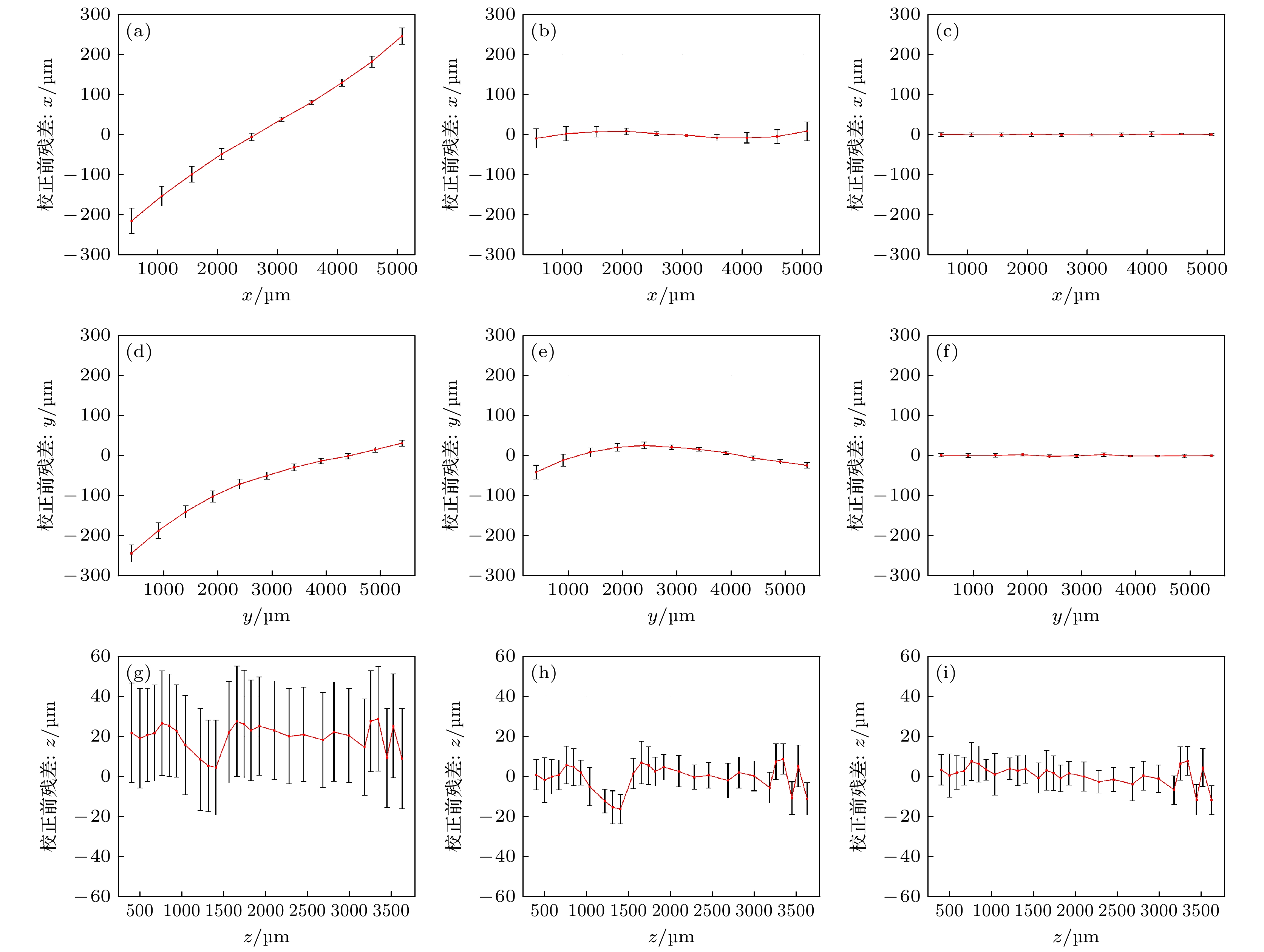
图 6 模型校正与真实点轴向残差与未校正对应真实点轴向残差分布图 (a), (d), (g)未校正点$P$与对应真实空间点$\hat P$坐标的X, Y, Z轴向残差; (b), (e), (h)线性回归模型的校正点$P'$与对应真实空间点$\hat P$坐标的X, Y, Z轴向残差; (c), (f), (i)本文校正模型的校正点$P'$与对应真实空间点$\hat P$坐标的X, Y, Z轴向残差
Fig. 6. Comparison of axial residuals between model-corrected data and true points versus uncorrected data and true points, along with their distribution plots: (a), (d), (g) Axial residuals (X/Y/Z) between uncorrected point $P$ and the ground-truth spatial point $\hat P$; (b), (e), (h) axial residuals (X/Y/Z) between the linear regression-corrected point $P'$ and the ground-truth spatial point $\hat P$; (c), (f), (i) axial residuals (X/Y/Z) between the proposed model-corrected point $P'$ and the ground-truth spatial point $\hat P$.
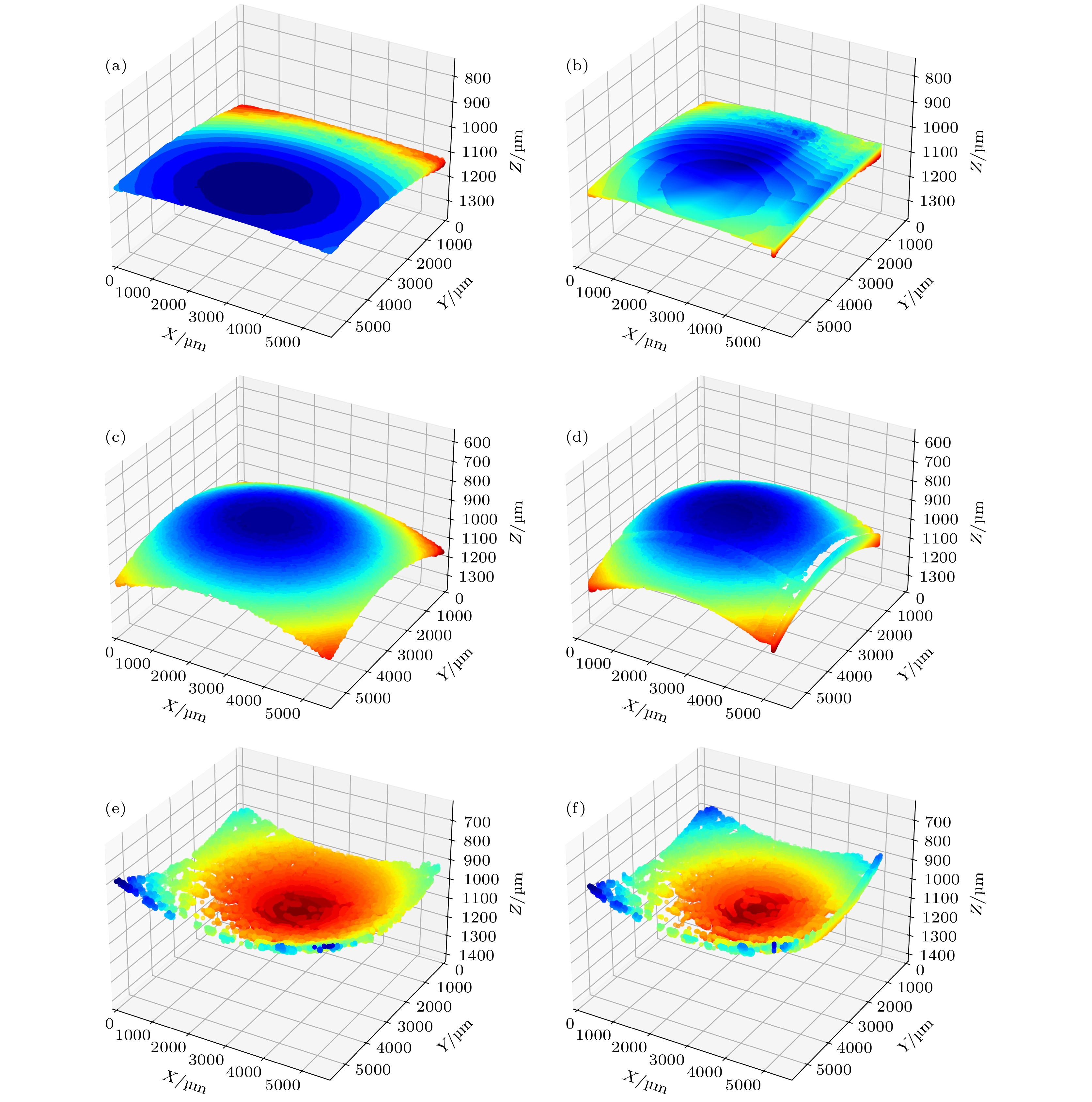
图 7 3种透镜第一面校正前后点云分布 (a)平凸透镜校正前; (b)平凸透镜校正后; (c)双凸透镜校正前; (d)双凸透镜校正后; (e)双凹透镜校正前; (f)双凹透镜校正后
Fig. 7. Point cloud distribution of the first surface of three types of lenses before and after correction: (a) Plano-convex lens before correction; (b) plano-convex lens after correction; (c) biconvex lens before correction; (d) biconvex lens after correction; (e) biconcave lens before correction; (f) biconcave lens after correction.
表 1 不同回归模型畸变校正效果
Table 1. Distortion correction performance of different regression models.
偏差值/μm $\Delta x$ $\Delta y$ $\Delta z$ $\Delta s$ 线性回归 11.92 18.68 9.85 40.45 K近邻 6.89 28.13 41.59 76.6 随机森林 19.16 14.36 99.12 132.64 XGBoost 6.68 45.19 54.18 106.05 本文方法 3.49 2.67 6.94 13.11 表 2 平凸透镜矫正前后参数测量结果对比
Table 2. Comparison of parameter measurement results for plano-convex lens before and after correction.
平凸透镜 R1 R2 d 校正前/mm 129.05 (45.71%/54.84%) — 1.334 (0.054%/4.2%) 校正后/mm 83.33 (0.01%/0.01%) — 1.288 (0.008%/0.6%) 名义标准值/mm –83.34 ∞ 1.28 表 3 双凸透镜矫正前后参数测量结果对比
Table 3. Comparison of parameter measurement results for biconvex lens before and after correction.
双凸透镜 R1 R2 d 校正前/mm 30.56 (6.01%/24.5%) 31.38 (6.83%/27.8%) 1.958 (0.48%/2.5%) 校正后/mm 24.58 (0.03%/0.1%) 24.73 (0.18%/0.7%) 1.918 (0.008%/0.4%) 名义标准值/mm –24.55 24.55 1.91 表 4 双凹透镜矫正前后参数测量结果对比
Table 4. Comparison of parameter measurement results for biconcave lens before and after correction.
双凹透镜 R1 R2 d 校正前/mm 29.87 (4.77%/19.0%) 18.93 (6.17%/24.6%) 0.927 (0.023%/2.4%) 校正后/mm 25.17 (0.07%/0.2%) 24.94 (0.16%/0.6%) 0.947 (0.003%/0.3%) 名义标准值/mm 25.10 –25.10 0.95 -
[1] Huang D, Swanson E A, Lin C P, Schuman J S, Stinson W G, Chang W, Hee M R, Flotte T, Gregory K, Puliafito C A, Fujimoto J G 1991 Science 254 1178
 Google Scholar
[2] Tomlins P H, Wang R K 2005 J. Phys. D Appl. Phys. 38 2519
 Google Scholar
[3] 丁宇韬, 张君, 郭遥, 陈昊 2024 激光与光电子学进展 61 247
Ding Y T, Zhang J, Guo Y, Chen H 2024 Laser Optoelectron. Prog. 61 247
[4] Volker W, Andrew R, Sunita R, Joseph I 2002 Opt. Express 10 397
 Google Scholar
[5] Diaz J, Rahlves M, Majdani O, Reithmeier E, Ortmaier T 2012 Optical Metrology and Inspection for Industrial Applications II Beijing, China, November 5–7, 2012 p8563J
[6] Yao J, Anderson A, Rolland J P 2018 Opt. Express 26 10242
 Google Scholar
[7] 江祥奎, 范永青, 王婉 2014 计算机科学与探索 8 1254
 Google Scholar
Jiang X Q, Fan Y Q, Wang W 2014 J. Front. Comput. Sci. Technol 8 1254
 Google Scholar
[8] 齐召帅, 王昭, 黄军辉, 薛琦, 高建民 2016 光子学报 45 87
Qi Z S, Wang Z, Huang J H, Xue Q, Gao J M 2016 Acta Photonica Sin. 45 87
[9] Lecun Y, Bottou L, Bengio Y, Haffner P 1998 Proc. IEEE 86 2278
 Google Scholar
[10] Li X Y, Zhang B, Sander P V, Liao J 2019 2019 IEEE/CVF Conference on Computer Vision and Pattern Recognition (CVPR) Long Beach, CA, USA, June 15–20, 2019 p4850
[11] Yang S R, Lin C Y, Liao K, Zhang C J, Zhao Y 2021 2021 IEEE/CVF Conference on Computer Vision and Pattern Recognition (CVPR) Nashville, TN, USA, June 20–25, 2021 p6344
[12] 徐启伟, 王佩佩, 曾镇佳, 黄泽斌, 周新星, 刘俊敏, 李瑛, 陈书青, 范滇元 2020 物理学报 69 014209
 Google Scholar
Xu Q W, Wang P P, Zeng Z J, Huang Z B, Zhou X X, Liu J M, Li Y, Chen S Q, Fan D Y 2020 Acta Phys. Sin. 69 014209
 Google Scholar
[13] 周静, 张晓芳, 赵延庚 2021 物理学报 70 054201
 Google Scholar
Zhou J, Zhang X F, Zhao Y G 2021 Acta Phys. Sin. 70 054201
 Google Scholar
[14] Shukla S, Vishwakarma C, Sah A N, Ahirwar S, Pandey K, Pradhan A 2023 Appl. Opt. 62 6826
 Google Scholar
[15] Breiman L, 2001 Mach. Learn. 45 5
 Google Scholar
[16] 谢探阳, 李玉梅, 张涛, 高天亮, 石玉超 2023 组合机床与自动化加工技术 2 37
Xie T Y, Li Y M, Zhang T, Gao T L, Shi Y C 2023 Mod. Mach. Tool Autom. Manuf. Tech. 2 37
[17] Kato D, Maeda N, Hirogaki T, Aoyama E, Takahashi K 2021 2021 21st International Conference on Control, Automation and Systems Jeju, Korea, October 12–15, 2021 p607
[18] Werbos P J 1981 System Modeling and Optimization Berlin, Germany, July 20–24, 1981 p762
[19] Rumelhart D E, Hinton G E, Williams R J 1986 Nature 323 533
 Google Scholar
[20] 杨沅松, 王晰, 任明俊 2023 光学学报 43 200
Yang Y S, Wang X, Ren M J 2023 Acta Opt. Sin. 43 200
[21] Singarimbun R N, Nababan E B, Sitompul O S 2019 2019 International Conference of Computer Science and Information Technology (ICoSNIKOM) Medan, Indonesia, November 28–29, 2019 p1
[22] Cotter A, Shamir O, Srebro N, Sridharan K 2011 Advances in Neural Information Processing Systems Granada, Spain, December 12–15, 2011 p1647
[23] Fitzgibbon A, Pilu M, Fisher R B 1999 IEEE Trans. Pattern Anal. Mach. Intell. 21 476
 Google Scholar
计量
- 文章访问数: 3783
- PDF下载量: 44
- 被引次数: 0


 下载:
下载:
