


-
The Talbot effect is a near-field diffraction effect that occurs in periodic structures. In a circular periodic structure with a point source as incident light, it has been found that there is no self-imaging effect of the grating at a certain propagation distance. In this paper, we combine the conformal transformation with the Talbot effect and work out a special medium in the physical space, which allows the circular grating to have a Talbot effect within it. The refractive index distribution generated by conformal transformation is calculated and the corresponding self-imaging radius expression is obtained. Lumerical product is used for simulation verification, and the applicable condition of the method is summarized. We separately carry out the simulations of a circular grating with and without the designed medium. Light field distributions in the two simulations differ from each other. The light field in the second situation shares more similarities with the light field of a plane grating than the first simulation. What is more, in the second situation, we can work out a certain Talbot radius, and the light field distribution at the calculated Talbot radius is quite similar to that at the circular grating. But for the first situation, we cannot calculate a certain Talbot radius and can obtain only the radius of the ring with highest self-imaging accuracy by comparing light field at each distance with the grating structure. We find that the small period of the circular grating we used in the second situation makes the light field at Talbot radius furcate. So we carry out a third simulation of a circular grating with a large period compared with the incident wavelength. The self-imaging result matches the grating structure quite well. However, there are some limits in this method. According to the conformal transformation, the refractive index near the center tends to be infinite, so we have to remove the medium near the center. Also, when the radius is big enough, refractive index there can be smaller than 1, so the Talbot effect should happen within this radius. In conclusion, we show that the transformation optics can be introduced into the self-imaging of circular gratings, and thus greatly expanding the range of applications for the Talbot effect.
-
Keywords:
- Talbot effect /
- self-imaging /
- circular grating /
- conformal transformation
[1] Talbot H F 1836 Philos. Mag. 9 401
[2] Rayleigh F R S 1881 Philos. Mag. 11 196
 Google Scholar
[3] Yashiro W, Harasse S, Takeuchi A, Suzuki Y, Momose A 2010 Phys. Rev. A 82 043822
[4] Zhang J, Chen Y 2015 Int. J. Nanotechnol. 12 917
[5] 周波, 陈云琳, 黎远安, 李海伟 2010 物理学报 59 1816
Google Scholar
Zhou B, Chen Y L, Li Y A, Li H W 2010 Acta Phys. Sin. 59 1816
Google Scholar
[6] 范天伟, 陈云琳, 张进宏 2013 物理学报 62 094216
Google Scholar
Fan T W, Chen Y L, Zhang J H 2013 Acta Phys. Sin. 62 094216
Google Scholar
[7] Côme Schnébelin, Chatellus H G D 2018 Opt. Lett. 43 1467
Google Scholar
[8] Candelas P, Fuster J M, Pérez-López S, Uris A, Rubio C 2019 Ultrasonics 94 281
Google Scholar
[9] Morozov A N, Krikunova M P, Skuibin B G, Smirnov E V 2017 JEPT Letters 106 23
[10] Kohn V G 2018 J. Synchrot. Radiat. 25 425
Google Scholar
[11] Kim J M, Cho I H, Lee S Y, Kang H C, Conley R, Liu C A, Macrander A T, Noh D Y 2010 Opt. Express 18 24975
Google Scholar
[12] Li C, Zhou T, Zhai Y, Yue X, Xiang J, Yang S, Wei X, Chen X 2017 Phys. Rev. A 95 033821
Google Scholar
[13] Li C, Zhou T, Xiang J, Zhai Y, Yue X, Yang S, Wei X, Chen X 2017 Chin. Phys. Lett. 34 084207
Google Scholar
[14] Pendry J B, Schurig D, Smith D R 2006 Science 312 1780
Google Scholar
[15] Leonhardt U 2006 Science 312 1777
Google Scholar
[16] 刘一超 2016 博士学位论文 (杭州: 浙江大学)
Liu Y C 2016 Ph. D. Dissertation (Hangzhou: Zhejiang University) (in Chinese)
[17] 徐林 2016 硕士学位论文 (苏州: 苏州大学)
Xu L 2016 M. S. Thesis (Suzhou: Suzhou University) (in Chinese)
[18] Wang X Y, Chen H Y, Liu H, Xu L, Sheng C, Zhu S N 2017 Phys. Rev. Lett. 119 033902
Google Scholar
[19] Torcal-Milla F J, Sanchez-Brea L M, Salgado-Remacha F J, Bernabeu E 2010 Opt. Commun. 283 3869
Google Scholar
[20] Zhang W, Wang J H, Cui Y W, Teng S Y 2015 Opt. Commun. 341 245
Google Scholar
[21] 乐阳阳 2016 硕士学位论文 (南京: 南京大学)
Yue Y Y 2016 M. S. Thesis (Nanjing: Nanjing University) (in Chinese)
[22] Xu L, Chen H Y 2015 Nat. Photon. 9 15
Google Scholar
-
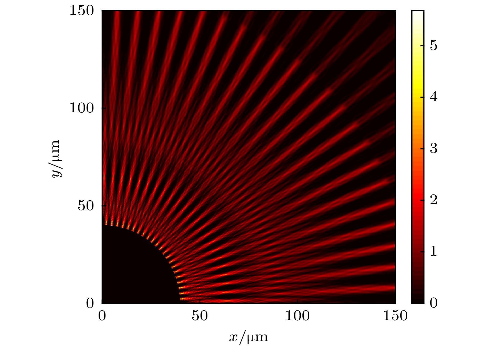
图 2 Lumerical模拟结果(光栅内的光场已去除)
Fig. 2. Simulation results (light field inside the grating has been removed).
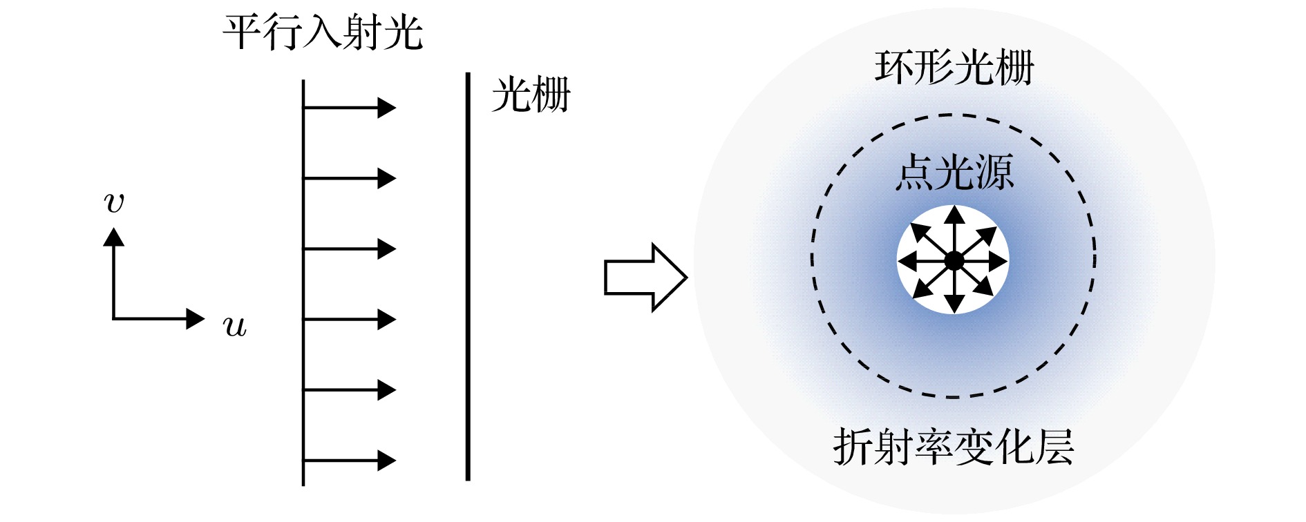
图 3 虚拟空间(左)和物理空间(右)示意图
Fig. 3. Schematic diagram of virtual space(left) and physical space(right).

图 4 对于内径为10 μm, 外径为10.1 μm, m = 50,
$m'$ = 50 μm的光栅, (a) Lumerical模拟结果(光栅内的光场已去除), 以及(b)自成像光场(短划线)与光栅处光场(实线)的对比Fig. 4. For the grating with the inner diameter of 10 μm and the outter diameter of 10.1 μm (m=50,
$m'$ = 50 μm), (a) simulation results (light field inside the grating has been removed), and (b) comparison of self-image (dash line) and the light field at r = 10.1 μm (solid line).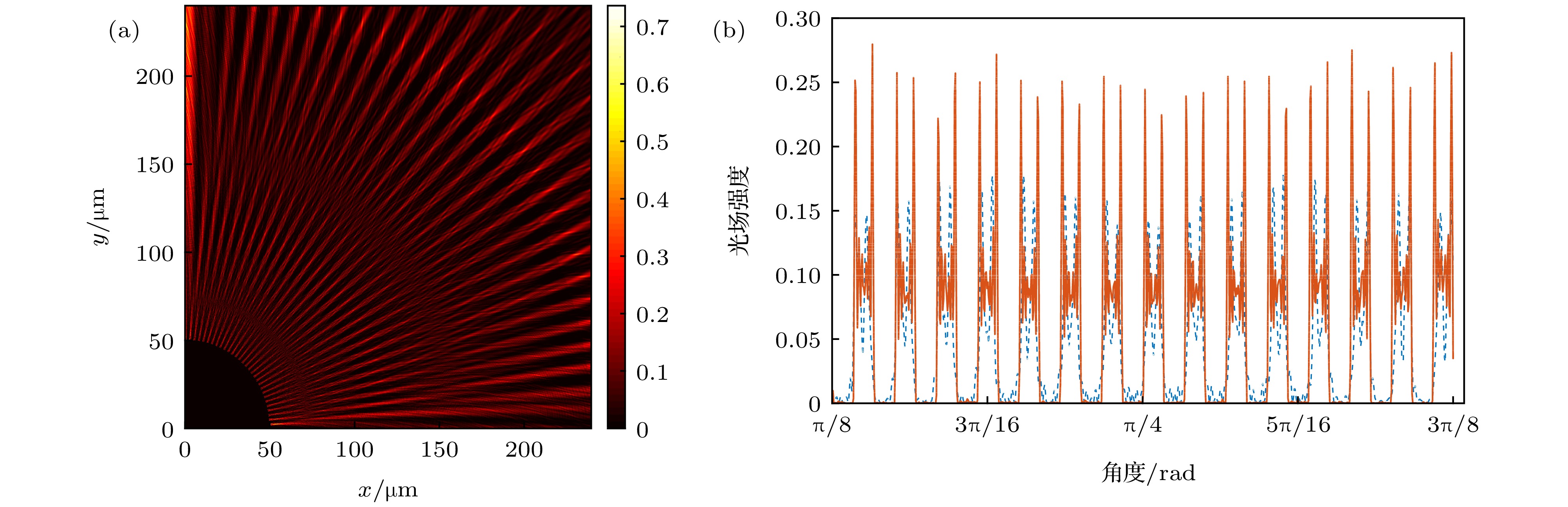
图 5 对于内径为50 μm, 外径为50.1 μm, m=120,
$m'$ = 300 μm的光栅, (a) Lumerical模拟结果(光栅内的光场已去除), 以及(b)自成像光场(虚线)与光栅处光场(实线)的对比Fig. 5. For the grating with the inner diameter of 50 μm and the outter diameter of 50.1 μm (m=120,
$m'$ = 300 μm), (a) simulation results (light field inside the grating has been removed), and (b) comparison of self-image (dash line) and the light field at r = 10.1 μm (solid line). -
[1] Talbot H F 1836 Philos. Mag. 9 401
[2] Rayleigh F R S 1881 Philos. Mag. 11 196
Google Scholar
[3] Yashiro W, Harasse S, Takeuchi A, Suzuki Y, Momose A 2010 Phys. Rev. A 82 043822
[4] Zhang J, Chen Y 2015 Int. J. Nanotechnol. 12 917
[5] 周波, 陈云琳, 黎远安, 李海伟 2010 物理学报 59 1816
Google Scholar
Zhou B, Chen Y L, Li Y A, Li H W 2010 Acta Phys. Sin. 59 1816
Google Scholar
[6] 范天伟, 陈云琳, 张进宏 2013 物理学报 62 094216
Google Scholar
Fan T W, Chen Y L, Zhang J H 2013 Acta Phys. Sin. 62 094216
Google Scholar
[7] Côme Schnébelin, Chatellus H G D 2018 Opt. Lett. 43 1467
Google Scholar
[8] Candelas P, Fuster J M, Pérez-López S, Uris A, Rubio C 2019 Ultrasonics 94 281
Google Scholar
[9] Morozov A N, Krikunova M P, Skuibin B G, Smirnov E V 2017 JEPT Letters 106 23
[10] Kohn V G 2018 J. Synchrot. Radiat. 25 425
Google Scholar
[11] Kim J M, Cho I H, Lee S Y, Kang H C, Conley R, Liu C A, Macrander A T, Noh D Y 2010 Opt. Express 18 24975
Google Scholar
[12] Li C, Zhou T, Zhai Y, Yue X, Xiang J, Yang S, Wei X, Chen X 2017 Phys. Rev. A 95 033821
Google Scholar
[13] Li C, Zhou T, Xiang J, Zhai Y, Yue X, Yang S, Wei X, Chen X 2017 Chin. Phys. Lett. 34 084207
Google Scholar
[14] Pendry J B, Schurig D, Smith D R 2006 Science 312 1780
Google Scholar
[15] Leonhardt U 2006 Science 312 1777
Google Scholar
[16] 刘一超 2016 博士学位论文 (杭州: 浙江大学)
Liu Y C 2016 Ph. D. Dissertation (Hangzhou: Zhejiang University) (in Chinese)
[17] 徐林 2016 硕士学位论文 (苏州: 苏州大学)
Xu L 2016 M. S. Thesis (Suzhou: Suzhou University) (in Chinese)
[18] Wang X Y, Chen H Y, Liu H, Xu L, Sheng C, Zhu S N 2017 Phys. Rev. Lett. 119 033902
Google Scholar
[19] Torcal-Milla F J, Sanchez-Brea L M, Salgado-Remacha F J, Bernabeu E 2010 Opt. Commun. 283 3869
Google Scholar
[20] Zhang W, Wang J H, Cui Y W, Teng S Y 2015 Opt. Commun. 341 245
Google Scholar
[21] 乐阳阳 2016 硕士学位论文 (南京: 南京大学)
Yue Y Y 2016 M. S. Thesis (Nanjing: Nanjing University) (in Chinese)
[22] Xu L, Chen H Y 2015 Nat. Photon. 9 15
Google Scholar


 下载:
下载:


计量
- 文章访问数: 15356
- PDF下载量: 119
- 被引次数: 0
