


-
研究非牛顿流体转捩问题, 可为调控非牛顿流体动力特性提供理论基础. 相对于牛顿流体转捩问题, 非牛顿流体转捩研究较少, 缺乏转捩雷诺数精细预报方法. 论文以格子Boltzmann方法为核心求解器, 以典型非牛顿流体幂律模型为例, 开展了幂律流体二维顶盖驱动流转捩模拟, 给出剪切变稀和剪切增稠流体的第一转捩雷诺数, 并分析了转捩雷诺数附近流场时频域特性及模态分布. 结果表明, 剪切变稀流体和剪切增稠流体的第一转捩雷诺数与牛顿流体差异显著, 且在转捩临界雷诺数附近监控点处速度分量均呈现周期性变化趋势. 通过对流场速度和涡量的本征正交分解发现, 不同类型的流体在转捩临界雷诺数附近, 前两阶模态均为流场的主模态, 能量占比超过95%, 且同类型流体不同雷诺数的主模态间具有相似的结构.
-
关键词:
- 幂律流体 /
- 转捩 /
- 格子Boltzmann方法 /
- 顶盖驱动流
Studying transitions from laminar to turbulence of non-Newtonian fluids can provide a theoretical basis to further mediate their dynamic properties. Compared with Newtonian fluids, transitions of non-Newtonian fluids turning are less focused, thus being lack of good predictions of the critical Reynolds number (Re) corresponding to the first Hopf bifurcation. In this study, we employ the lattice Boltzmann method as the core solver to simulate two-dimensional lid-driven flows of a typical non-Newtonian fluid modeled by the power rheology law. Results show that the critical Re of shear-thinning (5496) and shear-thickening fluids (11546) are distinct from that of Newtonian fluids (7835). Moreover, when Re is slightly larger than the critical one, temporal variations of velocity components at the monitor point all show a periodic trend. Before transition of the flow filed, the velocity components show a horizontal straight line, and after transition , the velocity components fluctuate greatly and irregularly. Through fast Fourier transform for the velocity components, it is noted that the velocity has a dominant frequency and a harmonic frequency when Re is marginally larger than the critical one. Besides, the velocity is steady before transition of flow filed, so it appears as a point on the frequency spectrum. As the flow filed turns to be turbulent, the frequency spectrum of the velocity component appears multispectral. Different from a single point in the velocity phase diagram before transition, the velocity phase diagram after transition forms a smooth and closed curve, whose area is also increasing as Re increases. The center point of the curve moves along a certain direction, while movement directions of different center points are different. Proper orthogonal decompositions for the velocity and vorticity field reveal that the first two modes, in all types of fluids, are the dominant modes when Re is close to the critical one, with energy, occupying more than 95% the whole energy. In addition, for one type of fluid, the dominant modes at different Re values have similar structures. Results of the first and second modes of velocity field show that the modal peak is mainly distributed in vicinity of the cavity wall.-
Keywords:
- power-law fluid /
- transition /
- lattice Boltzmann method /
- lid-driven flow
[1] Ghia U, Ghia K N, Shin C 1982 J. Comput. Phys. 48 387
 Google Scholar
[2] Yu H, Luo L S, Girimaji S S 2006 Comput. Fluids. 35 957
Google Scholar
[3] Lin L S, Chang H W, Lin C A 2013 Comput. Fluids. 80 381
Google Scholar
[4] Burggraf O R 1966 J. Fluid Mech. 24 113
Google Scholar
[5] Peng F, Shiau Y H, Hwang R R 2003 Comput. Fluids. 32 337
Google Scholar
[6] Bruneau C H, Saad M 2006 Comput. Fluids. 35 326
Google Scholar
[7] Auteri F, Parolini N, Quartapelle L 2002 J. Comput. Phys. 183 1
Google Scholar
[8] Sahin M, Owens R G 2003 Int. J. Numer. Methods Fluids 42 57
Google Scholar
[9] Gong X, Xu Y, Zhu W, Xuan S, Jiang W, Jiang W 2014 J. Compos Mater. 48 641
Google Scholar
[10] Giuntoli A, Puosi F, Leporini D, Starr F W, Douglas J F 2020 Sci. Adv. 6 eaaz0777
Google Scholar
[11] Johnston B M, Johnston P R, Corney S, Kilpatrick D 2004 J. Biomech. 37 709
Google Scholar
[12] Zhao C, Zholkovskij E, Masliyah J H, Yang C 2008 J. Colloid Interface Sci. 326 503
Google Scholar
[13] Hojjat M, Etemad S G, Bagheri R, Thibault J 2011 Int. Commun. Heat Mass Transf. 38 144
Google Scholar
[14] Chen S, Doolen G D 1998 Annu. Rev. Fluid Mech. 30 329
Google Scholar
[15] Shan X, Chen H 1993 Phys. Rev. E 47 1815
Google Scholar
[16] Hou S, Zou Q, Chen S, Doolen G, Cogley A C 1995 J. Comput. Phys. 118 329
Google Scholar
[17] He X, Chen S, Doolen G D 1998 J. Comput. Phys. 146 282
Google Scholar
[18] Boyd J, Buick J, Green S 2006 J. Phys. A: Math. Gen. 39 14241
Google Scholar
[19] Wang C H, Ho J R 2011 Comput. Math. Appl. 62 75
Google Scholar
[20] Chen Y L, Cao X D, Zhu K Q 2009 J. Non-Newtonian Fluid Mech. 159 130
Google Scholar
[21] Nejat A, Abdollahi V, Vahidkhah K 2011 J. Non-Newtonian Fluid Mech. 166 689
Google Scholar
[22] d'Humieres D 2002 Philos. Trans. Roy. Soc. A 360 437
Google Scholar
[23] Ren F, Song B, Zhang Y, Hu H 2018 Comput. Fluids. 173 29
Google Scholar
[24] Wei Y, Wang Z, Yang J, Dou H S, Qian Y 2015 Comput. Fluids. 118 167
Google Scholar
[25] Guo Z, Shi B, Wang N 2000 J. Comput. Phys. 165 288
Google Scholar
[26] Ziegler D P 1993 J. Stat. Phys. 71 1171
Google Scholar
[27] Yu D, Mei R, Shyy W 2003 41 st Aerospace Sciences Meeting and Exhibit Reno, USA, January 6−9, 1999 p953
[28] Gabbanelli S, Drazer G, Koplik J 2005 Phys. Rev. E 72 046312
Google Scholar
[29] Hall K C, Thomas J P, Dowell E H 2000 AIAA J. 38 1853
Google Scholar
[30] Taira K, Brunton S L, Dawson S T, et al. 2017 AIAA J. 55 4013
Google Scholar
[31] Cazemier W, Verstappen R, Veldman A 1998 Phys. Fluids 10 1685
Google Scholar
[32] Poliashenko M, Aidun C K 1995 J. Comput. Phys. 121 246
Google Scholar
-

图 2 LBM与幂律模型耦合计算流程示意图
Fig. 2. Diagram of coupling calculation process between LBM and power law model.
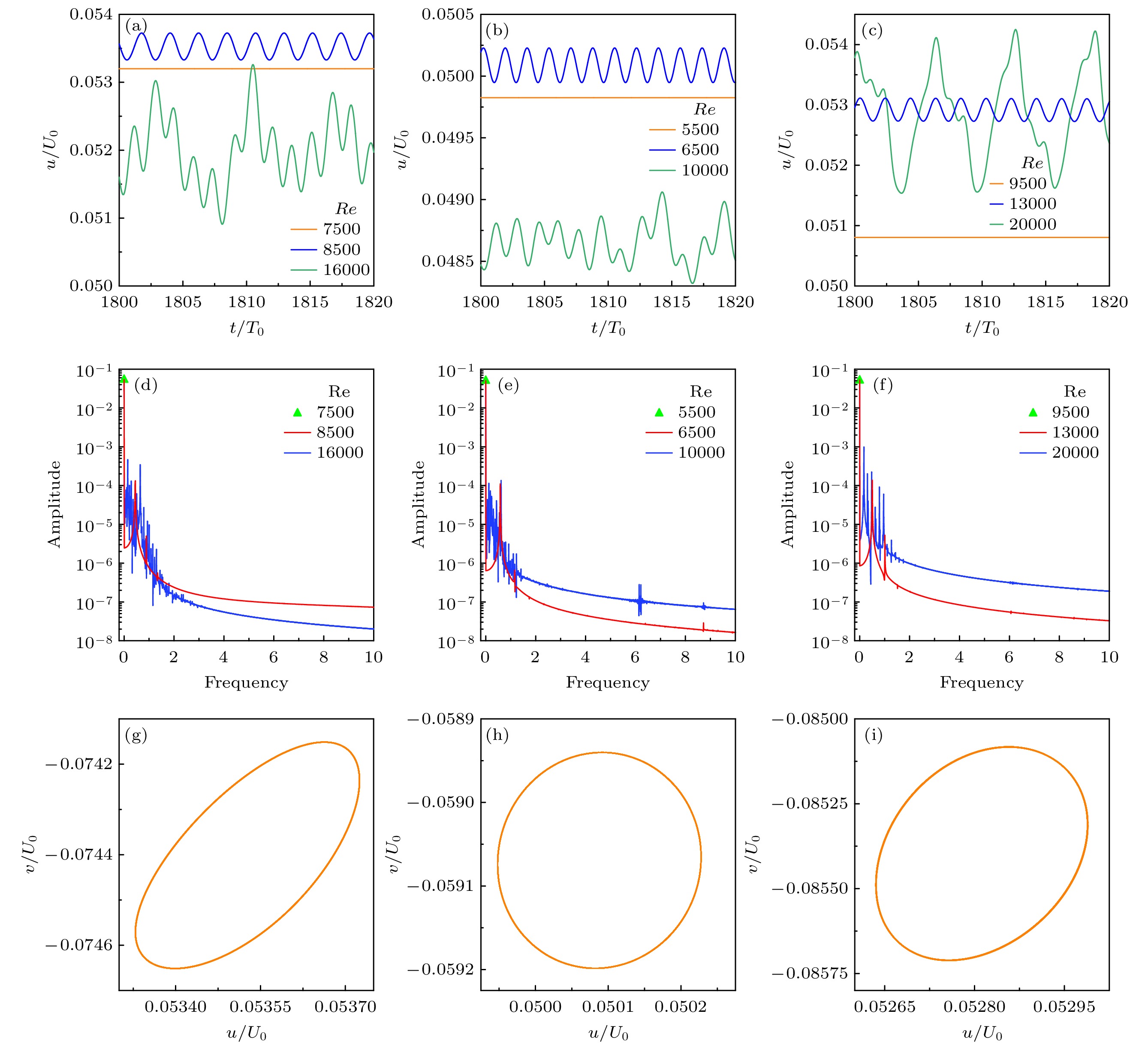
图 5 三类流体在速度监控点处的时频域特性 (a), (d) n = 1, Re = 7500, 8500, 16000; (g) n = 1, Re = 8500; (b), (e) n = 0.75, Re = 5500, 6500, 10000; (h) n = 0.75, Re = 6500; (c), (f) n = 1.25, Re = 9500, 13000, 20000; (i) n = 1.25, Re = 13000
Fig. 5. Time-frequency spectrum characteristics at the velocity monitoring point for three types of fluids: (a), (d) n = 1, Re = 7500, 8500, 16000; (g) n = 1, Re = 8500; (b), (e) n = 0.75, Re = 5500, 6500, 10000; (h) n = 0.75, Re = 6500; (c), (f) n = 1.25, Re = 9500, 13000, 20000; (i) n = 1.25, Re = 13000.
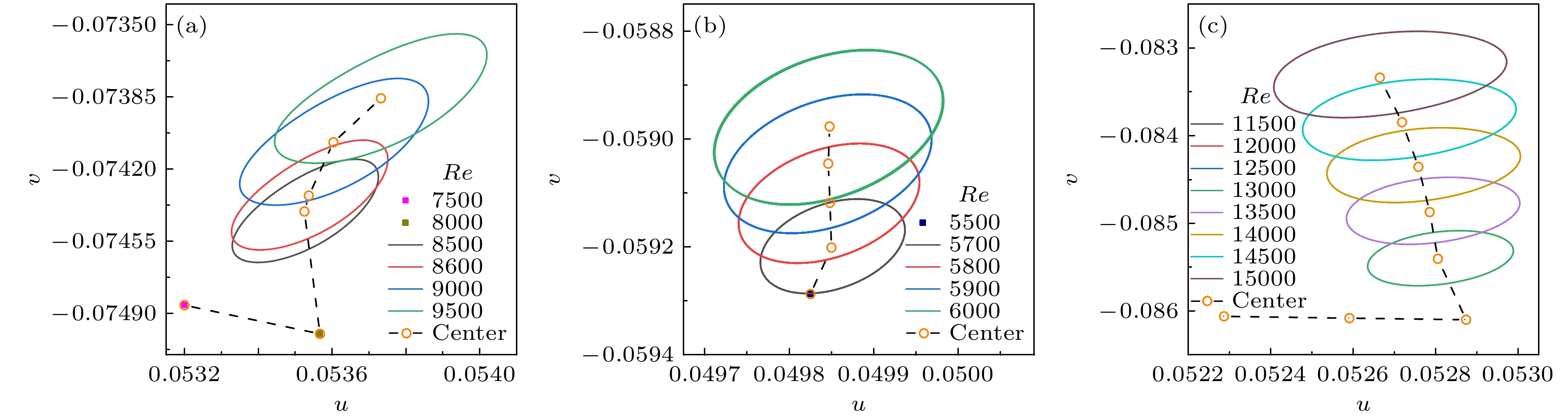
图 6 在监控点处的速度相图 (a) 牛顿流体; (b) 剪切变稀流体; (c) 剪切增稠流体
Fig. 6. Velocity phase diagrams at the monitoring point: (a) Newtonian fluid; (b) shear-thinning fluid; (c) shear-thickening fluid.
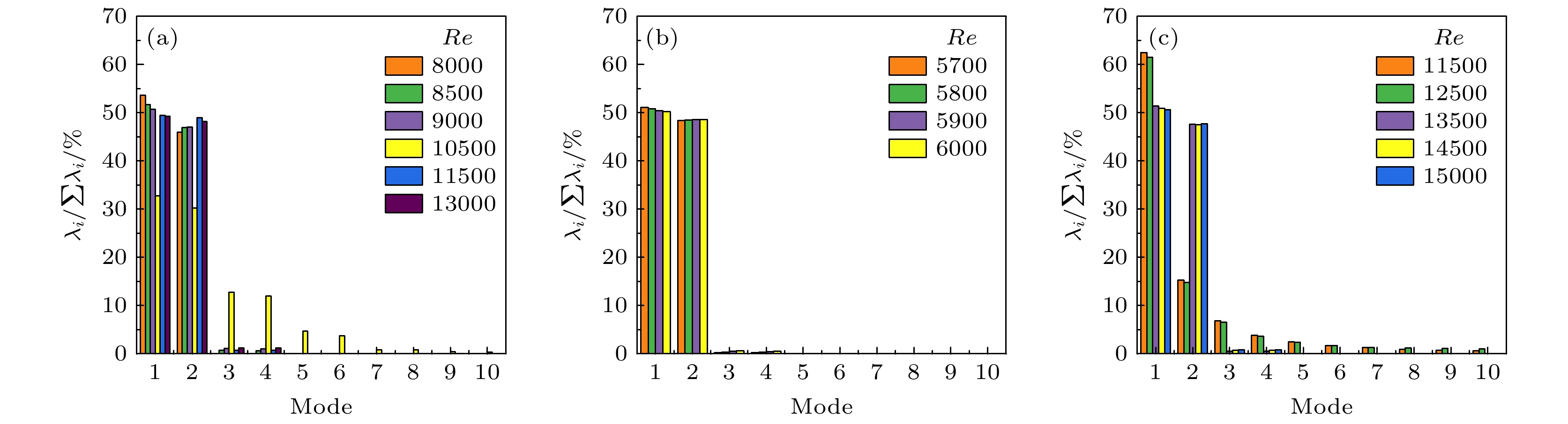
图 7 速度u的各阶模态的能量占比 (a) 牛顿流体; (b) 剪切变稀流体; (c) 剪切增稠流体
Fig. 7. Energy share of each order of mode for velocity u: (a) Newtonian fluid; (b) shear thinning-fluid; (c) shear-thickening fluid.
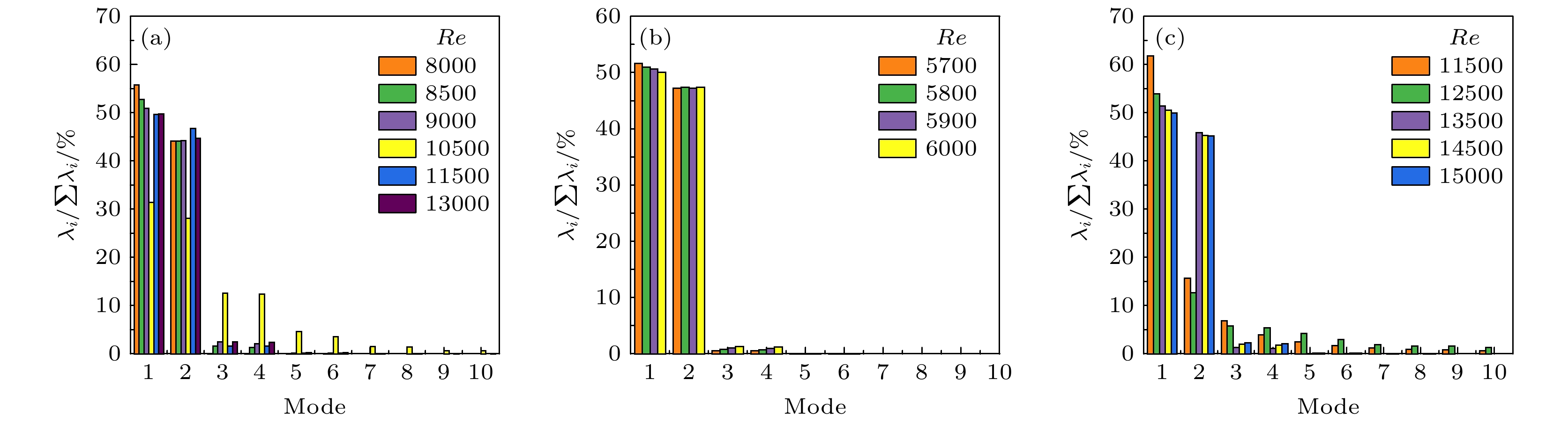
图 8 涡量的各阶模态的能量占比 (a) 牛顿流体; (b) 剪切变稀流体; (c) 剪切增稠流体
Fig. 8. Vortex energy share of each order of mode: (a) Newtonian fluid; (b) shear-thinning fluid; (c) shear-thickening fluid.

图 9 牛顿流体的水平速度的各阶模态图 (a), (b), (c) Re = 8500时, 平均场、一阶模态与二阶模态; (d), (e), (f) Re = 9000时, 平均场、一阶模态与二阶模态
Fig. 9. Modal diagrams of horizontal velocity of Newtonian fluid: (a), (b) and (c) The mean field, the first and second modes when Re = 8500; (d), (e), (f) mean field, first-order mode and second-order mode when Re = 9000
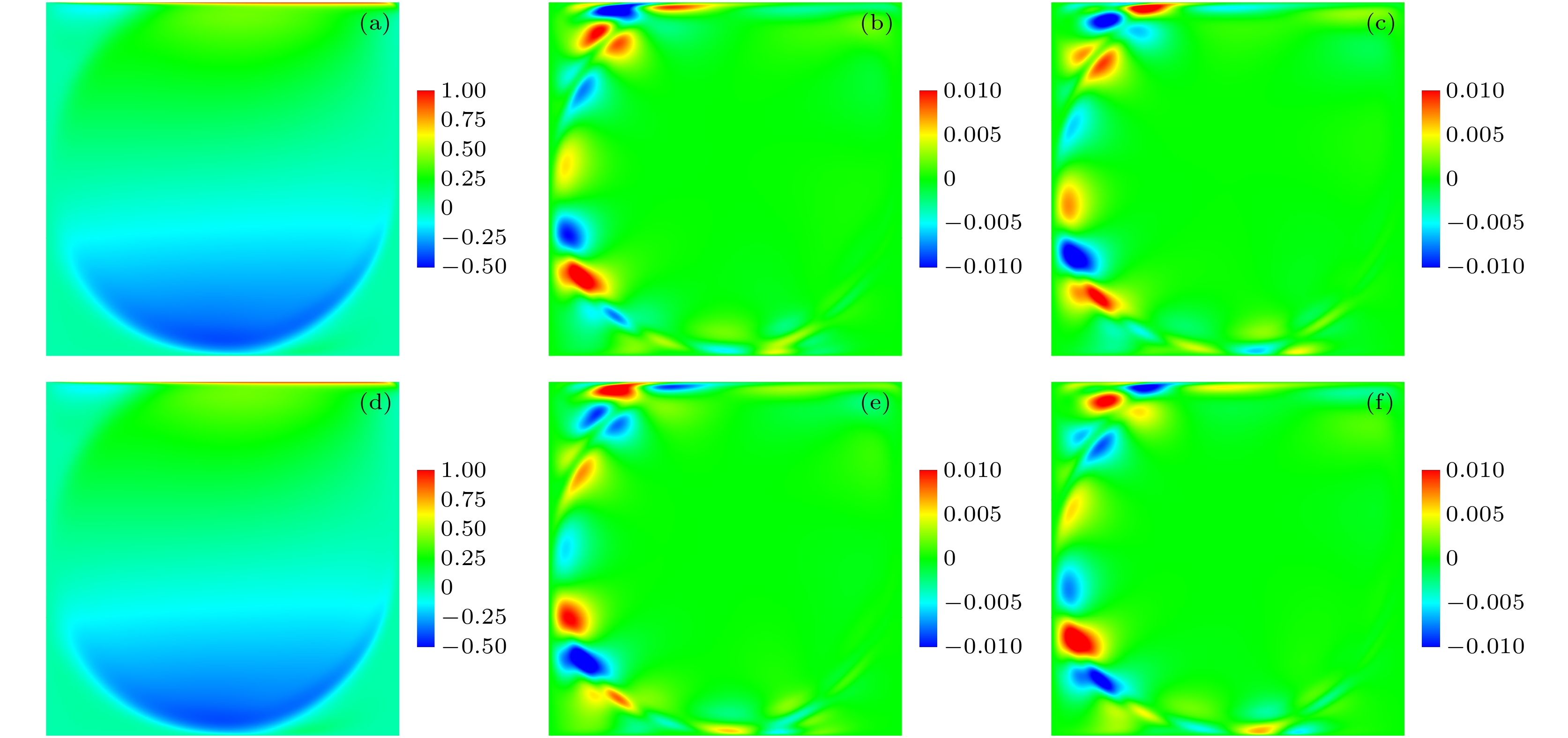
图 10 剪切变稀流体的水平速度的各阶模态图 (a), (b), (c) Re = 5700时, 平均场、一阶模态与二阶模态; (d), (e), (f) Re = 6000时, 平均场、一阶模态与二阶模态
Fig. 10. Modal diagrams of horizontal velocity of shear-thinning fluid: (a), (b), (c) The mean field, the first and second modes when Re = 5700; (d), (e), (f) mean field, first-order mode and second-order mode when Re = 6000.
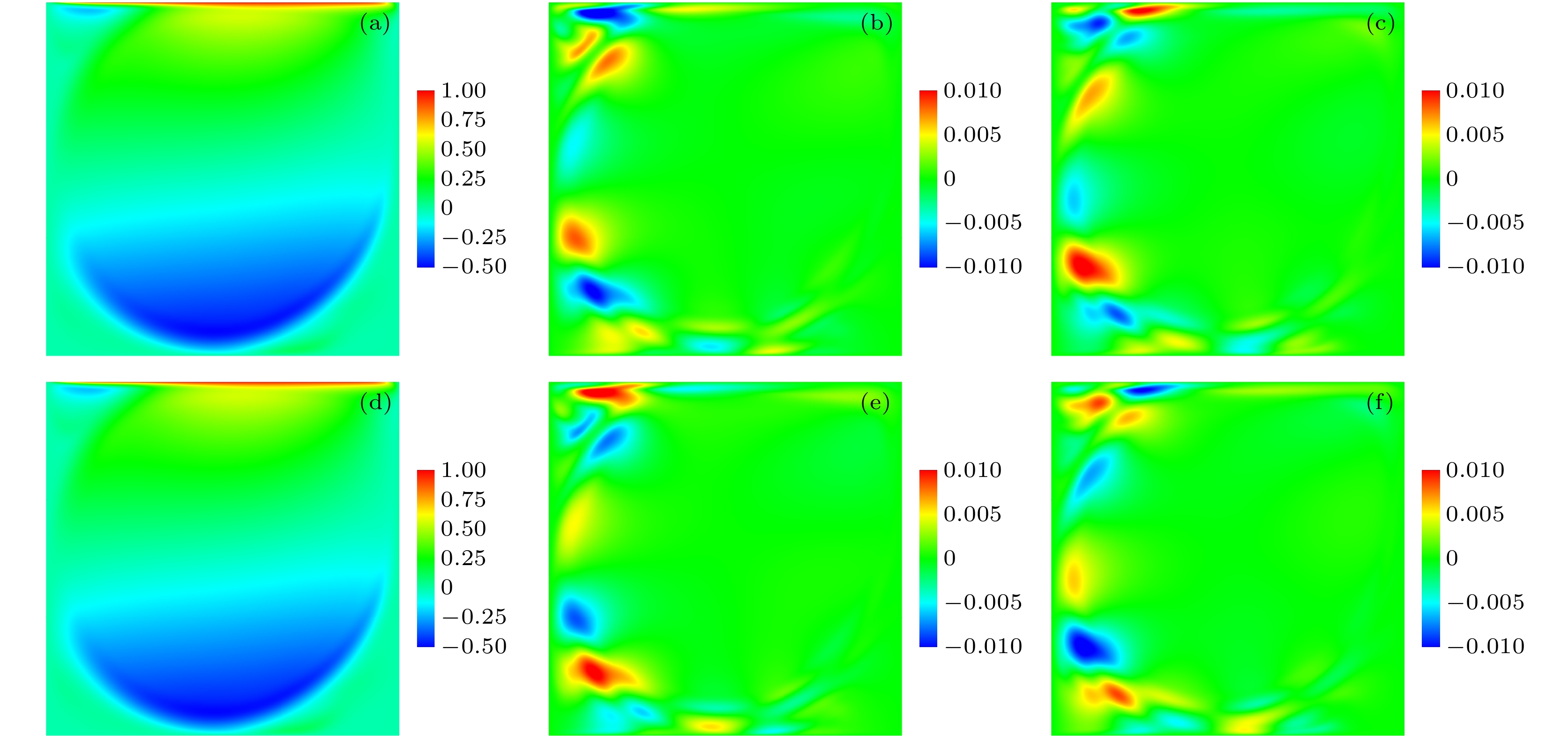
图 11 剪切增稠流体的水平速度的各阶模态图 (a), (b), (c) Re = 13000时, 平均场、一阶模态与二阶模态; (d), (e), (f) Re = 13500时, 平均场、一阶模态与二阶模态
Fig. 11. Modal diagrams of horizontal velocity of shear-thickening fluid: (a), (b), (c) The mean field, the first and second modes when Re = 13000; (d), (e), (f) mean field, first-order mode and second-order mode when Re = 13500.
-
[1] Ghia U, Ghia K N, Shin C 1982 J. Comput. Phys. 48 387
Google Scholar
[2] Yu H, Luo L S, Girimaji S S 2006 Comput. Fluids. 35 957
Google Scholar
[3] Lin L S, Chang H W, Lin C A 2013 Comput. Fluids. 80 381
Google Scholar
[4] Burggraf O R 1966 J. Fluid Mech. 24 113
Google Scholar
[5] Peng F, Shiau Y H, Hwang R R 2003 Comput. Fluids. 32 337
Google Scholar
[6] Bruneau C H, Saad M 2006 Comput. Fluids. 35 326
Google Scholar
[7] Auteri F, Parolini N, Quartapelle L 2002 J. Comput. Phys. 183 1
Google Scholar
[8] Sahin M, Owens R G 2003 Int. J. Numer. Methods Fluids 42 57
Google Scholar
[9] Gong X, Xu Y, Zhu W, Xuan S, Jiang W, Jiang W 2014 J. Compos Mater. 48 641
Google Scholar
[10] Giuntoli A, Puosi F, Leporini D, Starr F W, Douglas J F 2020 Sci. Adv. 6 eaaz0777
Google Scholar
[11] Johnston B M, Johnston P R, Corney S, Kilpatrick D 2004 J. Biomech. 37 709
Google Scholar
[12] Zhao C, Zholkovskij E, Masliyah J H, Yang C 2008 J. Colloid Interface Sci. 326 503
Google Scholar
[13] Hojjat M, Etemad S G, Bagheri R, Thibault J 2011 Int. Commun. Heat Mass Transf. 38 144
Google Scholar
[14] Chen S, Doolen G D 1998 Annu. Rev. Fluid Mech. 30 329
Google Scholar
[15] Shan X, Chen H 1993 Phys. Rev. E 47 1815
Google Scholar
[16] Hou S, Zou Q, Chen S, Doolen G, Cogley A C 1995 J. Comput. Phys. 118 329
Google Scholar
[17] He X, Chen S, Doolen G D 1998 J. Comput. Phys. 146 282
Google Scholar
[18] Boyd J, Buick J, Green S 2006 J. Phys. A: Math. Gen. 39 14241
Google Scholar
[19] Wang C H, Ho J R 2011 Comput. Math. Appl. 62 75
Google Scholar
[20] Chen Y L, Cao X D, Zhu K Q 2009 J. Non-Newtonian Fluid Mech. 159 130
Google Scholar
[21] Nejat A, Abdollahi V, Vahidkhah K 2011 J. Non-Newtonian Fluid Mech. 166 689
Google Scholar
[22] d'Humieres D 2002 Philos. Trans. Roy. Soc. A 360 437
Google Scholar
[23] Ren F, Song B, Zhang Y, Hu H 2018 Comput. Fluids. 173 29
Google Scholar
[24] Wei Y, Wang Z, Yang J, Dou H S, Qian Y 2015 Comput. Fluids. 118 167
Google Scholar
[25] Guo Z, Shi B, Wang N 2000 J. Comput. Phys. 165 288
Google Scholar
[26] Ziegler D P 1993 J. Stat. Phys. 71 1171
Google Scholar
[27] Yu D, Mei R, Shyy W 2003 41 st Aerospace Sciences Meeting and Exhibit Reno, USA, January 6−9, 1999 p953
[28] Gabbanelli S, Drazer G, Koplik J 2005 Phys. Rev. E 72 046312
Google Scholar
[29] Hall K C, Thomas J P, Dowell E H 2000 AIAA J. 38 1853
Google Scholar
[30] Taira K, Brunton S L, Dawson S T, et al. 2017 AIAA J. 55 4013
Google Scholar
[31] Cazemier W, Verstappen R, Veldman A 1998 Phys. Fluids 10 1685
Google Scholar
[32] Poliashenko M, Aidun C K 1995 J. Comput. Phys. 121 246
Google Scholar


 下载:
下载:

计量
- 文章访问数: 8042
- PDF下载量: 103
- 被引次数: 0
