基于统一流体模型的微放电数值仿真研究

王震; 赵志航; 付洋洋

doi:10.7498/aps.73.20240392

摘要

数值仿真技术已发展成为气体放电领域的重要研究手段, 常用于研究揭示某一具体放电形式的微观物理过程. 本文介绍了气体放电的统一流体模型, 包括粒子的连续性方程、能量守恒方程及泊松(Poisson)方程, 考虑阴极电子发射(二次电子、热电子发射)、反应焓变与气体加热、阴极热传导等基本过程, 可模拟得到包含盖革-米勒(Geiger-Müller)放电、汤森(Townsend)放电、辉光放电、电弧放电等各区域的完整伏安特性曲线. 基于该模型, 仿真得到的气体放电伏安特性曲线与已有文献结果一致, 验证了该模型的正确性. 在此基础上, 对间距为400 µm、气压分别为50和500 Torr (1 Torr ≈ 133.322 Pa)的放电过程进行了具体研究, 对比分析了不同气压条件下放电典型参量的分布特性. 该模型实现了广域参数范围条件下的气体放电数值仿真, 拓展了气体放电流体模型的应用范围, 促进了对放电参数特性的系统性分析.

关键词:

Abstract

Numerical simulation has become an indispensable tool in the study of gas discharge. However, it is typically used to reveal microscopic properties in a discharge under specific conditions. In this work, a unified fluid model for discharge simulation is introduced in detail. The model includes the continuity equation, the energy conservation equation of the species (electrons and heavy particles), and Poisson’s equation. The model takes into account some processes such as cathode electron emission (secondary electron emission and thermionic emission), reaction enthalpy change, gas heating, and cathode heat conduction. The full current-voltage characteristic (CVC) curve covers a range of discharge regimes, such as the Geiger-Müller discharge regime, Townsend discharge regime, subnormal glow discharge regime, normal glow discharge regime, abnormal glow discharge regime, and arc discharge regime. The obtained CVC curve is consistent with the results in the literature, confirming the validity of the unified fluid model. On this basis, the CVC curves are obtained in a wide pressure range of 50–3000 Torr. Simulation studies are carried out focusing on the discharge characteristics for microgap of 400 µm at pressures of 50 Torr and 500 Torr, respectively. The distributions of typical discharge parameters under different pressure conditions are analyzed by comparison. The results indicate that the electric field in the discharge gap is uniform, and that the space charge effect can be ignored in Townsend discharge regime. The cathode fall region and the quasi-neutral region both appear in glow discharge regime, and the space charge effect is significant. In particular, the electric field reversal occurs in abnormal discharge regime due to the heightened particle density gradient. The electron density reaches about 10²² m^–3 in arc discharge regime dominated by thermionic emission and thermal ionization, with the current density increasing. The gas temperature peak is 11850 K when the pressure is 500 Torr, and the cathode surface is heated to nearly 4000 K due to heat conduction. The present model can be used to simulate gas discharge across a wide range of condition parameters, promoting and expanding fluid model applications, and assisting in a more comprehensive investigation of discharge parameter properties.

Keywords:

作者及机构信息

清华大学电机工程与应用电子技术系, 北京　100084

通信作者: 付洋洋, fuyangyang@tsinghua.edu.cn

基金项目: 国家自然科学基金(批准号: 52277154)资助的课题.

Authors and contacts

Department of Electrical Engineering, Tsinghua University, Beijing 100084, China

Corresponding author: Fu Yang-Yang, fuyangyang@tsinghua.edu.cn

Funds: Project supported by the National Natural Science Foundation of China (Grant No. 52277154).

文章全文

参考文献

[1]	Hara K, Hanquist K 2018 Plasma Sources Sci. Technol. 27 065004 Google Scholar
[2]	Campanell M D, Johnson G R 2019 Phys. Rev. Lett. 122 015003 Google Scholar
[3]	Nanbu K 1980 J. Phys. Soc. Jpn. 49 2042 Google Scholar
[4]	Wilczek S, Schulze J, Brinkmann R P, Donkó Z, Trieschmann J, Mussenbrock T 2020 J. Appl. Phys. 127 181101 Google Scholar
[5]	Donkó Z, Derzsi A, Vass M, Horváth B, Wilczek S, Hartmann B, Hartmann P 2021 Plasma Sources Sci. Technol. 30 095017 Google Scholar
[6]	Petrović Z L, Škoro N, Marić D, Mahony C M O, Maguire P D, Radmilović-Rađenović M, Malović G 2008 J. Phys. D: Appl. Phys. 41 194002 Google Scholar
[7]	Yang D, Wang H H, Zheng B C, Zou X B, Wang X X, Fu Y Y 2023 Phys. Plasmas 30 063510 Google Scholar
[8]	Yang D, Wang H H, Zheng B C, Liu Z G, Fu Y Y 2023 Plasma Sources Sci. Technol. 32 10LT01 Google Scholar
[9]	付洋洋, 罗海云, 邹晓兵, 王强, 王新新 2014 物理学报 63 095206 Google Scholar Fu Y Y, Luo H Y, Zou X B, Wang Q, Wang X X 2014 Acta Phys. Sin. 63 095206 Google Scholar
[10]	Zhao Z H, Wei X L, Guan R Y, Nie H Y, Zhu B, Yao Y H 2022 IEEE Trans. Plasma Sci. 50 2333 Google Scholar
[11]	张晓宁, 李和平, Murphy A B, 夏维生 2013 高电压技术 39 7 Google Scholar Zhang X N, Li H P, Murphy A B, Xia W S 2013 High Voltage Eng. 39 7 Google Scholar
[12]	Surendra M, Graves D B, Jellum G M 1990 Phys. Rev. A 41 1112 Google Scholar
[13]	Fiala A, Pitchford L C, Boeuf J P 1994 Phys. Rev. E 49 5607 Google Scholar
[14]	Farouk T, Farouk B, Staack D, Gutsol A, Fridman A 2006 Plasma Sources Sci. Technol. 15 676 Google Scholar
[15]	Bogaerts A, Gijbels R, Goedheer W J 1996 Anal. Chem. 68 2296 Google Scholar
[16]	Liu X H, He W, Yang F, Wang H Y, Liao R J, Xiao H G 2012 Chin. Phys. B 21 075201 Google Scholar
[17]	Chen S, Nobelen J, Nijdam S 2017 Plasma Sources Sci. Technol. 26 095005 Google Scholar
[18]	Chen S, Li K, Nijdam S 2019 Plasma Sources Sci. Technol. 28 055017 Google Scholar
[19]	Wang L, Chen S, Wang F 2019 Plasma Chem. Plasma Process. 39 1291 Google Scholar
[20]	Liu F C, Guo X, Zhou Z X, He Y F, Fan W L 2019 Phys. Plasmas 26 123505 Google Scholar
[21]	Marić D, Hartmann P, Malović G, Donkó Z, Petrović Z L 2003 J. Phys. D: Appl. Phys. 36 2639 Google Scholar
[22]	Zhu Y F, Starikovskaia S 2018 Plasma Sources Sci. Technol. 27 124007 Google Scholar
[23]	Wu Y, Zhu Y F, Cui W, Jia M, Li Y H 2015 Plasma Processes Polym. 12 642 Google Scholar
[24]	Chen X C, Zhu Y F, Wu Y, Su Z, Liang H 2020 Plasma Processes Polym. 53 465202 Google Scholar
[25]	Babaeva N Y, Kushner M J 2009 J. Phys. D: Appl. Phys. 42 132003 Google Scholar
[26]	Babaeva N Y, Naidis G V 2016 Phys. Plasmas 23 083527 Google Scholar
[27]	Nijdam S, Teunissen J, Ebert U 2020 Plasma Sources Sci. Technol. 29 103001 Google Scholar
[28]	Luque A, Ratushnaya V, Ebert U 2008 J. Phys. D: Appl. Phys. 41 234005 Google Scholar
[29]	Yan W, Economou D J 2017 J. Phys. D: Appl. Phys. 50 415205 Google Scholar
[30]	Jiang Y Y, Wang Y H, Zhang J, Wang D Z 2022 J. Phys. D: Appl. Phys. 55 335203 Google Scholar
[31]	Kolobov V I, Fiala A 1994 Phys. Rev. E 50 3018 Google Scholar
[32]	Arslanbekov R R, Kolobov V I 2003 J. Phys. D: Appl. Phys. 36 2986 Google Scholar
[33]	Eliseev S I, Kudryavtsev A A, Liu H, Ning Z X, Yu D R, Chirtsov A S 2016 IEEE Trans. Plasma Sci. 44 2536 Google Scholar
[34]	Fu Y Y, Zhang P, Verboncoeur J P 2018 Appl. Phys. Lett. 112 254102 Google Scholar
[35]	Fu Y Y, Zhang P, Krek J, Verboncoeur J P 2019 Appl. Phys. Lett. 114 014102 Google Scholar
[36]	Fu Y Y, Wang H H, Zheng B C, Zhang P, Fan Q H, Wang X X, Verboncoeur J P 2021 Appl. Phys. Lett. 118 401 Google Scholar
[37]	Fu Y Y, Krek J, Zhang P, Verboncoeur J P 2018 IEEE Trans. Plasma Sci. 47 2011 Google Scholar
[38]	Chen J D, Verboncoeur J P, Fu Y Y 2022 Appl. Phys. Lett. 121 074102 Google Scholar
[39]	Baeva M, Loffhagen D, Uhrlandt D 2019 Plasma Chem. Plasma Process. 39 1359 Google Scholar
[40]	Baeva M, Loffhagen D, Becker M M, Uhrlandt D 2019 Plasma Chem. Plasma Process. 39 949 Google Scholar
[41]	Baeva M, Uhrlandt D, Loffhagen D 2020 Jpn. J. Appl. Phys. 59 SHHC05 Google Scholar
[42]	Saifutdinov A I, Fairushin I I, Kashapov N F 2016 JETP Lett. 104 180 Google Scholar
[43]	Saifutdinov A I 2021 J. Appl. Phys. 129 093302 Google Scholar
[44]	Saifutdinov A I 2022 Plasma Sources Sci. Technol. 31 094008 Google Scholar
[45]	王大智, 袁博文, 卢琪, 乔俊杰, 熊青 2023 电工技术学报 38 09 Google Scholar Wang D Z, Yuan B W, Lu Q, Qiao J J, Xiong Q 2023 Trans. China Electrotech. Soc. 38 09 Google Scholar
[46]	Bogaerts A, Gijbels R 1999 J. Appl. Phys. 86 4124 Google Scholar
[47]	Hayashi M 2003 Bibliography of Electron and Photon Cross Sections with Atoms and Molecules published in the 20th century (Toki, Gifu: National Inst. for Fusion Science) NIFS-DATA-72
[48]	Cunningham A J, O’Malley T F, M H R 1981 J. Phys. B: At. Mol. Phys. 14 773 Google Scholar
[49]	Jonkers J, Sande M van de, Sola A, Gamero A, Rodero A, Mullen J van der 2003 Plasma Sources Sci. Technol. 12 464 Google Scholar
[50]	Niu C, Hu Y H, Shao K, Sun S R, Wang H X 2022 Plasma Chem. Plasma Process. 42 885 Google Scholar
[51]	Kolokolov N B, Kudrjavtsev A A, Blagoev A B 1994 Phys. Scr. 50 371 Google Scholar
[52]	Lymberopoulos D P, Economou D J 1993 J. Appl. Phys. 73 3668 Google Scholar
[53]	Karoulina E V, Lebedev Y A 1992 J. Phys. D: Appl. Phys. 25 401 Google Scholar
[54]	Kannari F, Suda A, Obara M, Fujioka T 1983 IEEE J. Quantum Electron. 19 1587 Google Scholar
[55]	Gregório J, Leprince P, Boisse-Laporte C, Alves L L 2012 Plasma Sources Sci. Technol. 21 015013 Google Scholar
[56]	Rafatov I, Bogdanov E A, Kudryavtsev A A 2012 Phys. Plasmas 19 033502 Google Scholar
[57]	Kolokolov N B, Blagoev A B 1993 Phys.-Usp. 36 152 Google Scholar
[58]	Beulens J J, Milojevic D, Schram D C, Vallinga P M 1991 Phys. Fluids B 3 2548 Google Scholar
[59]	杜世刚 1998 等离子体物理 (北京: 原子能出版社) 第160—163页 Du S G 1998 Plasma Physics (Beijing: Atomic Press) pp160–163
[60]	Bird R B, Steward W E, Lightfoot E N 2001 Transport Phenomena (Hoboken: Wiley) p526
[61]	Chapman S, Cowling T G 1995 The Mathematical Theory of Non-uniform Gases: an Account of the Kinetic Theory of Viscosity, Thermal Conduction and Diffusion in Gases (Cambridge: Cambridge university Press) p167
[62]	张东荷雨, 刘金宝, 付洋洋 2024 物理学报 73 025201 Google Scholar Zhang D H Y, Liu J B, Fu Y Y 2024 Acta Phys. Sin. 73 025201 Google Scholar
[63]	Brokaw R S 1969 Ind. Eng. Chem. Process Des. Dev. 8 240 Google Scholar
[64]	Neufeld P D, Janzen A R, Aziz R A 1972 J. Chem. Phys. 57 1100 Google Scholar
[65]	Gurvich L V, Veyts I V, Alcock C B 1989 Thermodynamic Properties of Individual Substances (Vol. 1) (4th Ed.) (Washington: Hemisphere Publishing Corp) pp135–138
[66]	Maltsev M A, Morozov I V, Osina E L 2019 High Temp. 57 37 Google Scholar
[67]	刘富成, 晏雯, 王德真 2013 物理学报 62 175204 Google Scholar Liu F C, Yan W, Wang D Z 2013 Acta Phys. Sin. 62 175204 Google Scholar
[68]	Incropera F P, DeWitt D P, Bergmann T L, Lavine A S 2007 Fundamentals of Heat and Mass Transfer (New York: John Wiley) p68
[69]	Touloukian Y S, Powell R W, Ho C Y, Clemens P G 1970 Thermal Conductivity: Metallic Tlements and Alloys (Thermophysical Properties of Matter) (New York: Plenum Press) pp415−428
[70]	Brown S B 1959 Basic Data of Plasma Physics (New York: John Wiley and Sons, Inc.) pp167–211
[71]	Schottky W 1914 Ann. Phys. 44 1011 Google Scholar
[72]	杨津基 1983 气体放电 (北京: 科学出版社) 第50页 Yang J J 1983 Gas Discharge (Beijing: Science Press) p50
[73]	邵先军, 马跃, 李娅西, 张冠军 2010 物理学报 59 8747 Google Scholar Shao X J, Ma Y, Li Y X, Zhang G J 2010 Acta Phys. Sin. 59 8747 Google Scholar
[74]	COMSOL AB, Stockholm, Sweden COMSOL Multiphysics^® v.6.1
[75]	Si Ma W X, Peng Q J, Yang Q, Yuan T, Shi J 2012 IEEE Trans. Dielectr. Electr. Insul. 19 660 Google Scholar
[76]	Zhuang Y, Chen G, Rotaru M 2011 J. Phys: Conference Series 310 012011 Google Scholar
[77]	Raizer Y P 1991 Gas Discharge Physics (Berlin: Springer-Verlag) pp167–211
[78]	Gudmundsson J T, Hecimovic A 2017 Plasma Sources Sci. Technol. 26 123001 Google Scholar
[79]	Paschen F 1889 Ann. Phys. 273 69 Google Scholar
[80]	徐学基, 诸定昌 1996 气体放电物理 (上海: 复旦大学出版社) 第121—126页 Xu X J, Zhu D C 1996 Gas Discharge Physics (Shanghai: Fudan University Press) pp121–126
[81]	Townsend J S 1900 Nature 62 340 Google Scholar
[82]	岳清宇, 金花 1988 辐射防护 6 1 Yue Q Y, Jin H 1988 Radiat. Prot. 6 1
[83]	Lü B, Wang X X, Luo H Y, Liang Z 2009 Chin. Phys. B 18 646 Google Scholar
[84]	梁曦东, 周远翔, 曾嵘 2015 高电压工程(第2版) (北京: 清华大学出版社) 第17, 18页 Liang X D, Zhou Y X, Zeng R 2015 High Voltage Engineering (2nd Ed.) (Beijing: Tsinghua University Press) pp17, 18
[85]	Bouchikhi A, Hamid A 2010 Plasma Sci. Technol. 12 59 Google Scholar
[86]	Levko D, Subramaniam V, Raja L L 2022 Phys. Plasmas 29 023503 Google Scholar
[87]	Bogaerts A, Neyts E, Gijbels R, Van der M J 2002 Spectrochim. Acta, Part B 57 609 Google Scholar
[88]	Bogaerts A, Gijbels R, Goedheer W J 1995 J. Appl. Phys. 78 2233 Google Scholar
[89]	姚聪伟, 马恒驰, 常正实, 李平, 穆海宝, 张冠军 2017 物理学报 66 025203 Google Scholar Yao C W, Ma H C, Chang Z S, Li P, Mu H B, Zhang G J 2017 Acta Phys. Sin. 66 025203 Google Scholar
[90]	Montie T C, Kelly-Wintenberg K, Roth J R 2000 IEEE Trans. Plasma Sci. 28 41 Google Scholar
[91]	Gottscho R A, Mitchell A, Scheller G R, Chan Y Y, Graves D B 1989 Phys. Rev. A 40 6407 Google Scholar
[92]	Wang Q, Economou D J, Donnelly V M 2006 J. Appl. Phys. 100 023301 Google Scholar
[93]	Kolobov V I, Tsendin L D 1992 Phys. Rev. A 46 7837 Google Scholar
[94]	Boeuf J P, Pitchford L C 1995 J. Phys. D: Appl. Phys. 28 2083 Google Scholar
[95]	Kudryavtsev A A, Toinova N E 2005 Tech. Phys. Lett. 31 370 Google Scholar
[96]	Kudryavtsev A A, Nisimov S U, Prokhorova E I, Slyshov A G 2011 Tech. Phys. Lett. 37 838 Google Scholar
[97]	Kudryavtsev A A, Nisimov S U, Prokhorova E I, Slyshov A G 2012 Tech. Phys. 57 1188 Google Scholar
[98]	Barzilovich K A, Bogdanov E A, Kudryavtsev A A 2014 Tech. Phys. Lett. 40 581 Google Scholar
[99]	Marić D, Kutasi K, Malović G, Petrović Z L 2002 Eur. Phys. J. D 21 73 Google Scholar
[100]	Phelps A V 2001 Plasma Sources Sci. Technol. 10 329 Google Scholar
[101]	Franklin R N 2003 J. Phys. D: Appl. Phys. 36 R309 Google Scholar

施引文献

图 1 氩气直流微放电结构示意图. 其中, 电极间距$L_\text{gap} = 400\;{\text{μm}}$, 电极半径$R_\text{el} = 2\; {\text{mm}}$, 阴极导体材料为钨, 长度$L_\text{cath} = $$ 20 \;{\text{mm}}$

Fig. 1. Schematic diagram of the Ar DC microdischarge. The gap distance between the anode and cathode is $L_\text{gap} = 400\;{\text{μm}}$. The radius of electrodes is $R_\text{el} = 2\; {\text{mm}}$. The cathode is tungsten and it’s length is $L_\text{cath} = 20 \;{\text{mm}}$.

下载: 全尺寸图片幻灯片

图 2 阴极材料(钨)的比热容$C_\text{p,M}$、导热率$ \kappa_\text{M} $、发射率$ \epsilon_\text{M}$随温度的变化

Fig. 2. Specific heat capacity ($C_\text{p, M}$), thermal conductivity ($ \kappa_\text{M} $), and emissivity ($ \epsilon_\text{M}$) of tungsten cathode scaling with temperature.

下载: 全尺寸图片幻灯片

图 3 不同参数条件下得到的放电CVC曲线　(a) $p_0 = $$ 760 \;\text{Torr} \;(1 \;\text{atm})$条件下, 本文模拟结果与文献[40]结果对比; (b) $p_0 = 760 \;\text{Torr}$条件下, 电阻扫描与电压扫描所得CVC曲线结果一致, 具体放电模式取决于外电路$V{\text{-}}I$曲线与CVC曲线的交点; (c)气压分别为$p_1 = 50 \;\text{Torr}$, $p_2 = $$ 500 \;\text{Torr}$时, 仿真得到的CVC曲线

Fig. 3. CVC curves of the microdischarges under different conditions: (a) Benchmark between the calculation results of the unified fluid model in this article with the Ref. [40] at $p_0$ = 760 Torr; (b) overlapping CVC curves obtained by ballast resistor sweeping and voltage source sweeping at $p_\text{0}$ = 760 Torr, the discharge regime depends on the intersection of external circuit $V{\text{-}}I$ curves and the CVC curve; (c) CVC curves at $p_\text{1} = 50 \;\text{Torr}$ and $p_\text{2} = 500 \;\text{Torr}$.

下载: 全尺寸图片幻灯片

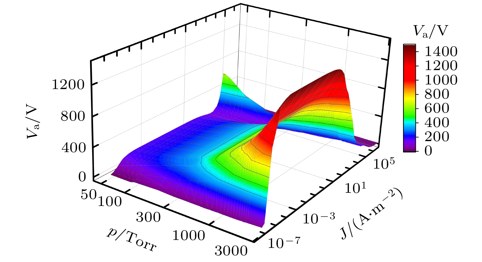
图 4 气压在50—3000 Torr范围内得到的CVC曲线

Fig. 4. The CVC curves obtained with the gas pressure ranging from 50 Torr to 3000 Torr.

下载: 全尺寸图片幻灯片

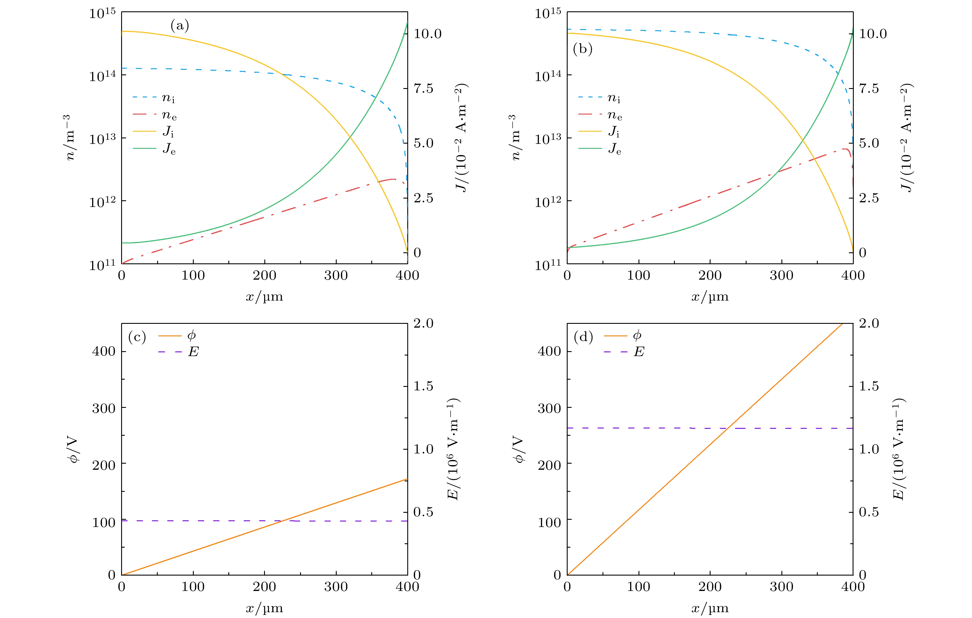
图 5 汤森放电区的参数特性($x = 0$的位置为阴极, $x = 400\; \text{μm}$的位置为阳极)　(a) p₁ = 50 Torr 与 (b) p₂ = 500 Torr条件下电子密度($n_\text{e}$)、离子密度($n_\text{i}=n_{\text{Ar}^+} + n_{\text{Ar2}^+}$)、电子电流密度($J_\text{e}$)、离子电流密度($J_\text{i}$)的空间分布; (c) p₁ = 50 Torr 与 (d) p₂ = 500 Torr条件下电势(ϕ)和电场(E)的空间分布

Fig. 5. Discharge characteristics in Townsend discharge regime. The position of $x = 0$ is the cathode and $x = 400\;{\text{μm}}$ is the anode. Spatial distributions of the electron density ($n_\text{e}$), ion density ($n_\text{i}=n_{\text{Ar}^+} + n_{\text{Ar2}^+}$), electron current density ($J_\text{e}$), and ion current density ($J_\text{i}$) at (a) 50 Torr and (b) 500 Torr. The corresponding spatial distributions of the electric potential (ϕ) and the electric field (E) at (c) 50 Torr and (d) 500 Torr.

下载: 全尺寸图片幻灯片

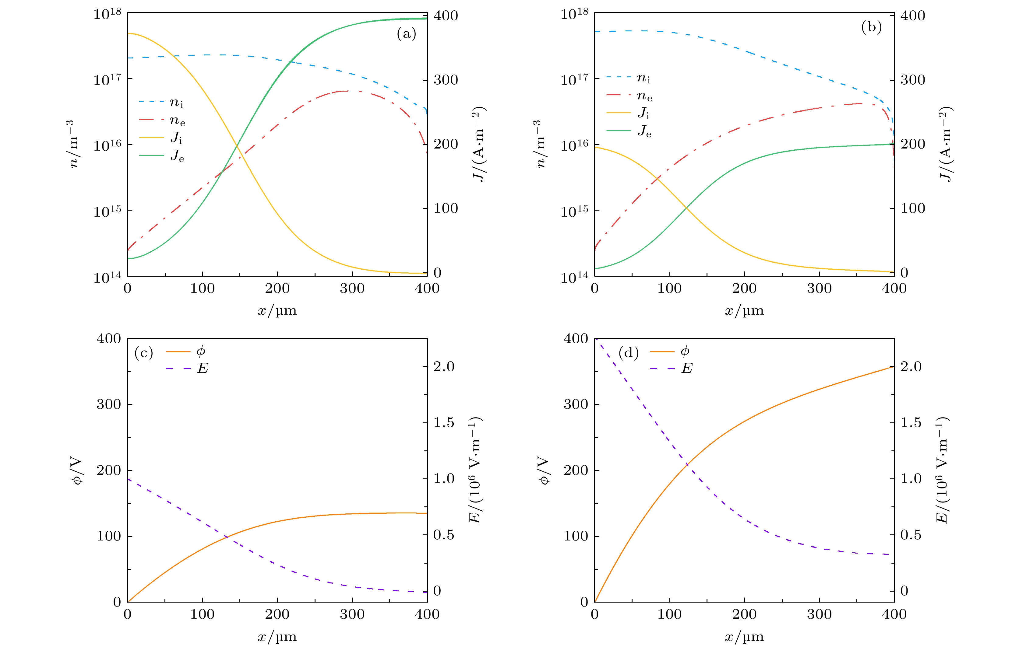
图 6 亚正常辉光放电区的参数特性　(a) p₁ = 50 Torr 与 (b) p₂ = 500 Torr条件下电子密度($n_\text{e}$)、离子密度($n_\text{i}$)、电子电流密度($J_\text{e}$)、离子电流密度($J_\text{i}$)的空间分布; (c) p₁ = 50 Torr 与 (d) p₂ = 500 Torr条件下电势(ϕ)和电场(E)的空间分布

Fig. 6. Discharge characteristics in subnormal glow discharge regime. Spatial distributions of the electron density ($n_\text{e}$), ion density ($n_\text{i}$), electron current density ($J_\text{e}$), and ion current density ($J_\text{i}$) at (a) 50 Torr and (b) 500 Torr. The corresponding spatial distributions of the electric potential (ϕ) and the electric field (E) at (c) 50 Torr and (d) 500 Torr.

下载: 全尺寸图片幻灯片

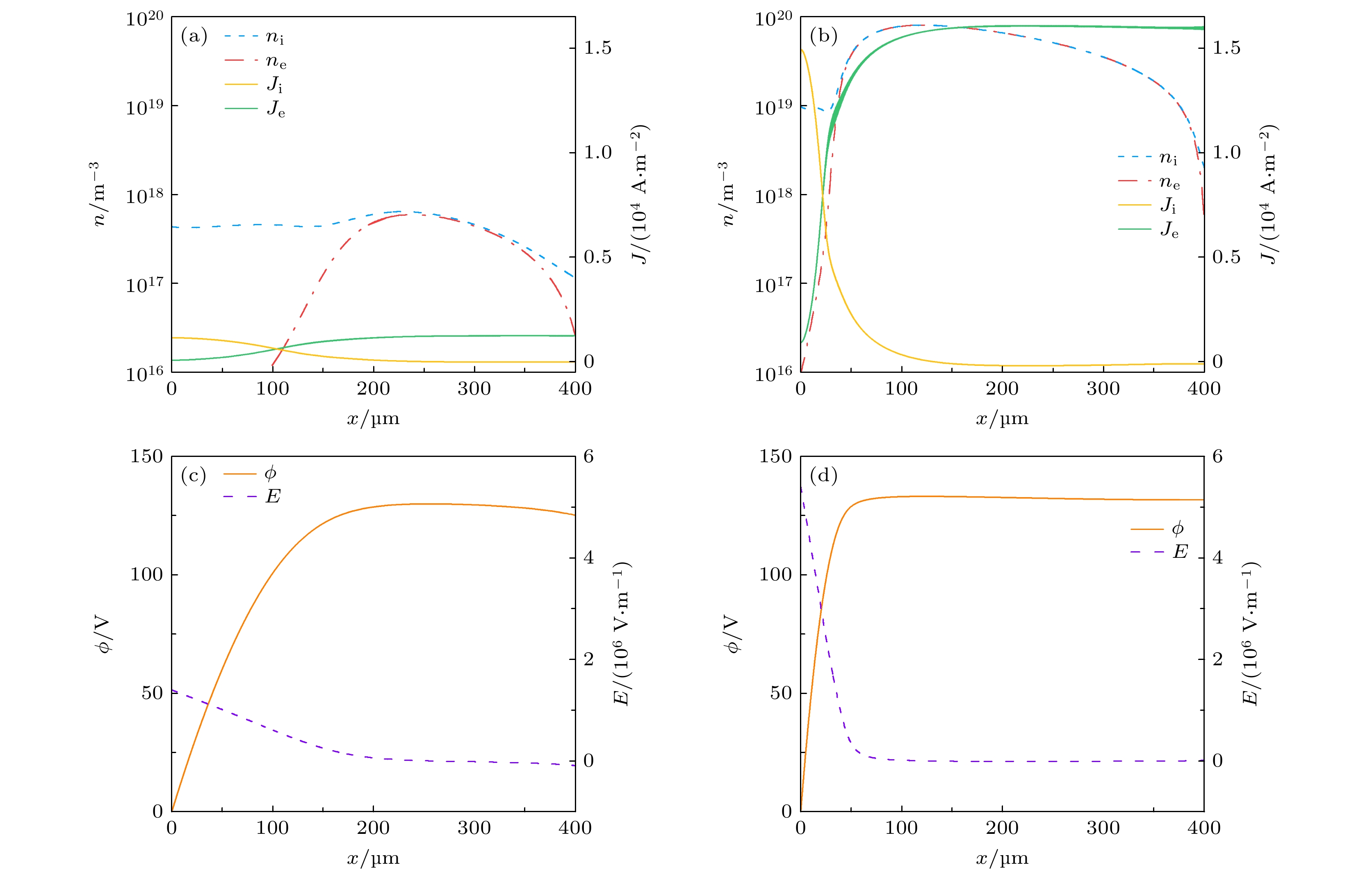
图 7 正常辉光放电区的参数特性　(a) p₁ = 50 Torr 与 (b) p₂ = 500 Torr条件下电子密度($n_\text{e}$)、离子密度($n_\text{i}$)、电子电流密度($J_\text{e}$)、离子电流密度($J_\text{i}$)的空间分布; (c) p₁ = 50 Torr 与 (d) p₂ = 500 Torr条件下电势(ϕ)和电场(E)的空间分布

Fig. 7. Discharge characteristics in normal glow discharge regime. Spatial distributions of the electron density ($n_\text{e}$), ion density ($n_\text{i}$), electron current density ($J_\text{e}$), and ion current density ($J_\text{i}$) at (a) 50 Torr and (b) 500 Torr. The corresponding spatial distributions of the electric potential (ϕ) and the electric field (E) at (c) 50 Torr and (d) 500 Torr.

下载: 全尺寸图片幻灯片

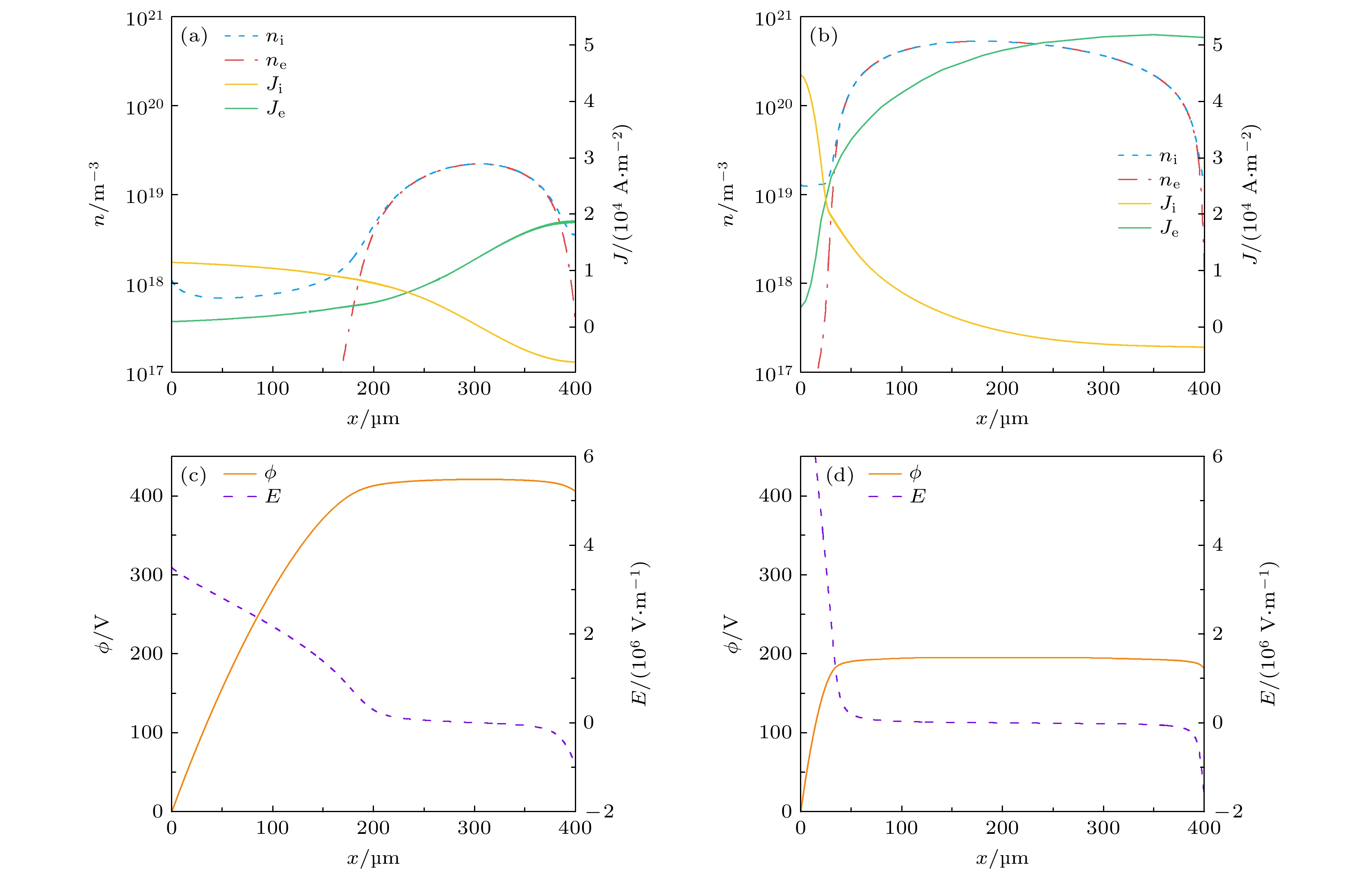
图 8 反常辉光放电区的参数特性　(a) p₁ = 50 Torr 与 (b) p₂ = 500 Torr条件下电子密度($n_\text{e}$)、离子密度($n_\text{i}$)、电子电流密度($J_\text{e}$)、离子电流密度($J_\text{i}$)的空间分布; (c) p₁ = 50 Torr 与 (d) p₂ = 500 Torr条件下电势(ϕ)和电场(E)的空间分布

Fig. 8. Discharge characteristics in abnormal glow discharge regime. Spatial distributions of the electron density ($n_\text{e}$), ion density ($n_\text{i}$), electron current density ($J_\text{e}$), and ion current density ($J_\text{i}$) at (a) 50 Torr and (b) 500 Torr. The corresponding spatial distributions of the electric potential (ϕ) and the electric field (E) at (c) 50 Torr and (d) 500 Torr.

下载: 全尺寸图片幻灯片

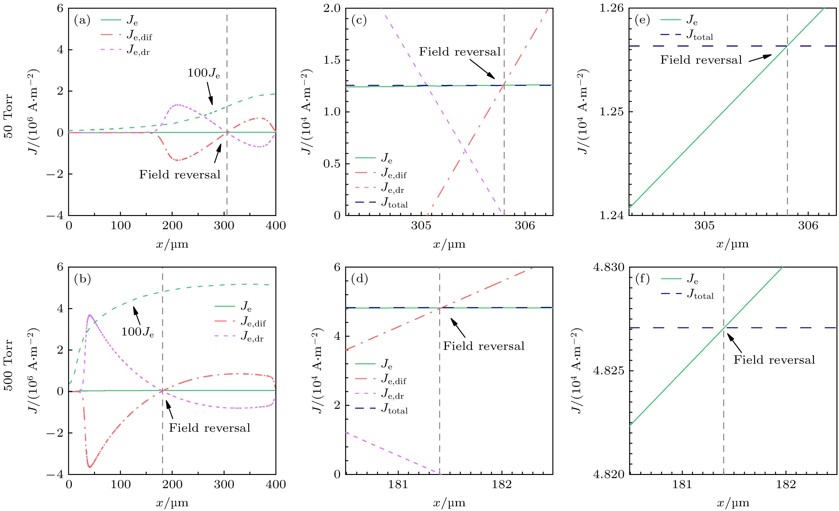
图 9 反常辉光放电区, (a) 50 Torr和(b) 500 Torr条件下电子电流密度($J_\text{e}$)、电子扩散电流密度($J_\text{e, dif}$)、电子漂移电流密度($J_\text{e, dr}$)的空间分布, 其中虚线为电场反转临界位置$x_\text{r}$; (c), (d)两个气压条件下电场反转临界位置附近的总电流密度($J_\text{total}$)与其他电流密度分量的空间分布; (e), (f)对应气压下电场反转临界位置的总电流密度与电子电流密度的空间分布

Fig. 9. Spatial distributions of the electron current density ($J_\text{e}$), the diffusion ($J_\text{e, dif}$), and the drift ($J_\text{e, dr}$) component of the electron current density in the abnormal glow regime at (a) 50 Torr and (b) 500 Torr. The dotted line is the critical position of the electric field reversal ($x_\text{r}$). Spatial distributions of total current density ($J_\text{total}$) and other current density components near the $x_\text{r}$ at (c) 50 Torr and (d) 500 Torr. Spatial distributions of the $J_\text{total}$ and $J_\text{e}$ near the $x_\text{r}$ at (e) 50 Torr and (f) 500 Torr.

下载: 全尺寸图片幻灯片

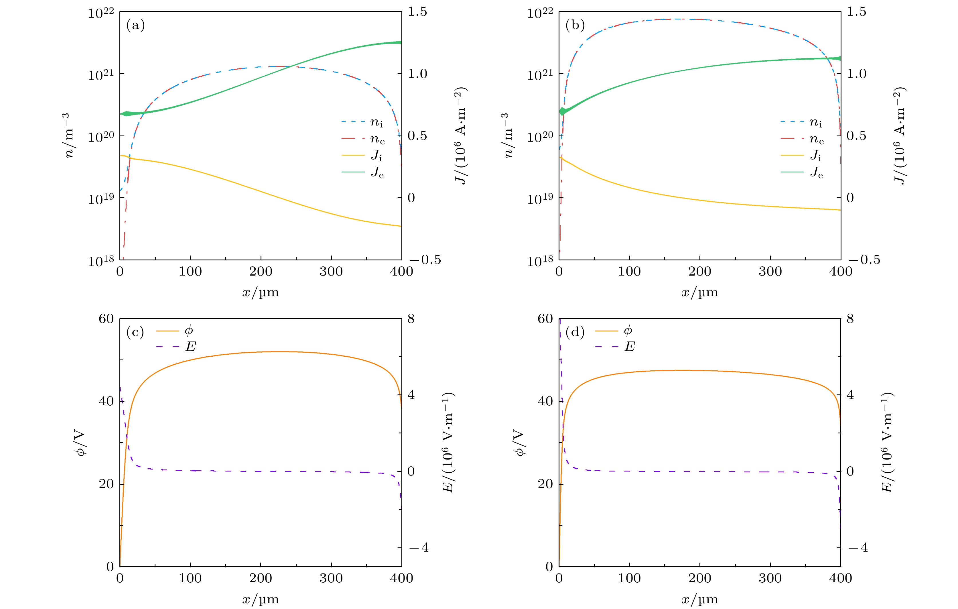
图 10 电弧放电区的参数特性　(a) p₁ = 50 Torr 与 (b) p₂ = 500 Torr条件下电子密度($n_\text{e}$)、离子密度($n_\text{i}$)、电子电流密度($J_\text{e}$)、离子电流密度($J_\text{i}$)的空间分布; (c) p₁ = 50 Torr 与 (d) p₂ = 500 Torr条件下电势(ϕ)和电场(E)的空间分布

Fig. 10. Discharge characteristics in arc discharge regime. Spatial distributions of the electron density ($n_\text{e}$), ion density ($n_\text{i}$), electron current density ($J_\text{e}$), and ion current density ($J_\text{i}$) at (a) 50 Torr and (b) 500 Torr. The corresponding spatial distributions of the electric potential (ϕ) and the electric field (E) at (c) 50 Torr and (d) 500 Torr.

下载: 全尺寸图片幻灯片

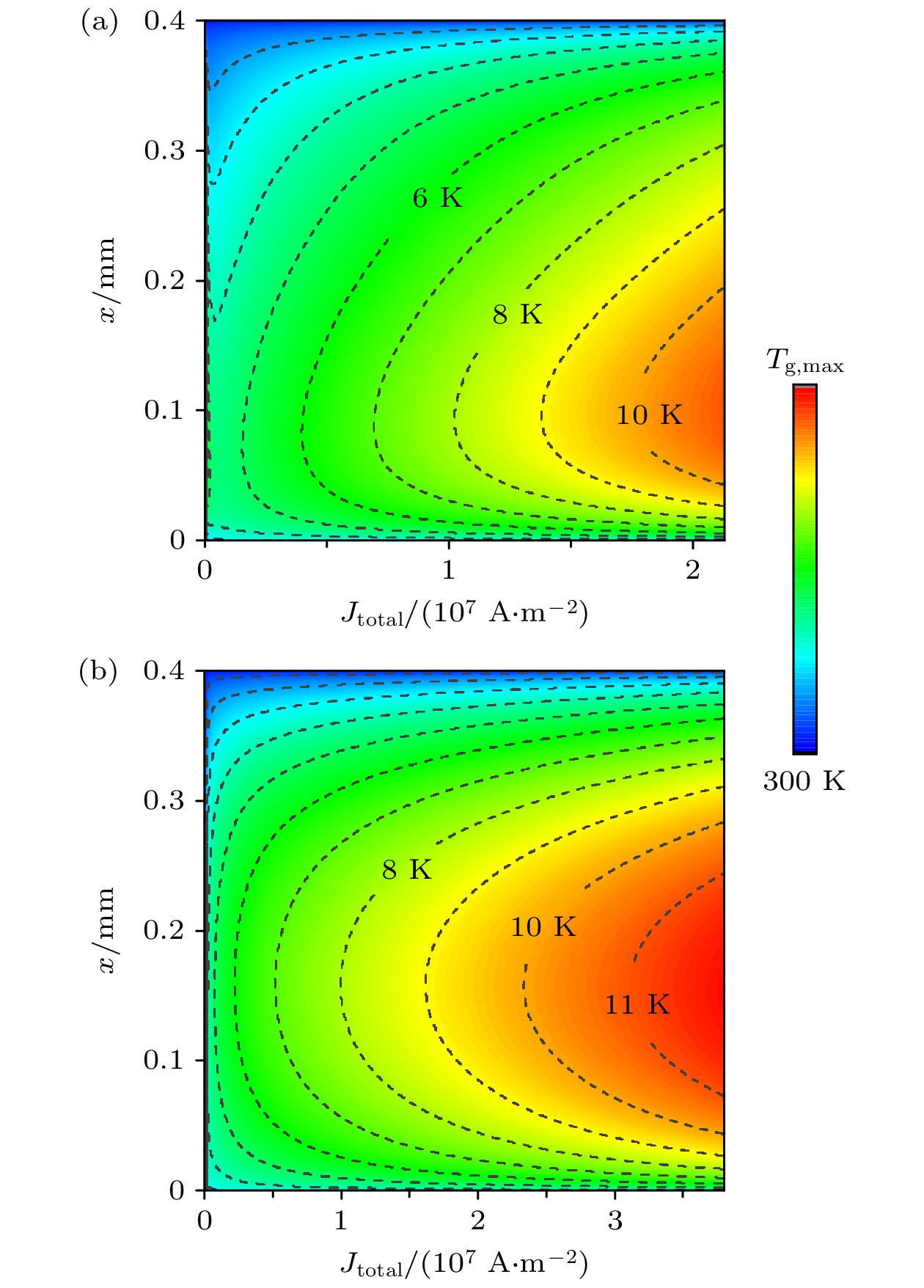
图 11 (a) 50 Torr和(b) 500 Torr条件下气体温度空间分布随放电电流密度的关系. 放电初始气体温度均为300 K, 其中, 500 Torr时, 气体温度最大值$T_\text{g,max} = 11850 \;\text{K}$

Fig. 11. Spatial distributions of discharge gap gas temperature scaling with current density at $p=$ (a) $50 \;\text{Torr}$ and (b) $500 \;\text{Torr}$. The initial temperature is 300 K. The maximum gas temperature ( $ T_\text{g,max} $ ) is 11850 K at $500 \;\text{Torr}$.

下载: 全尺寸图片幻灯片

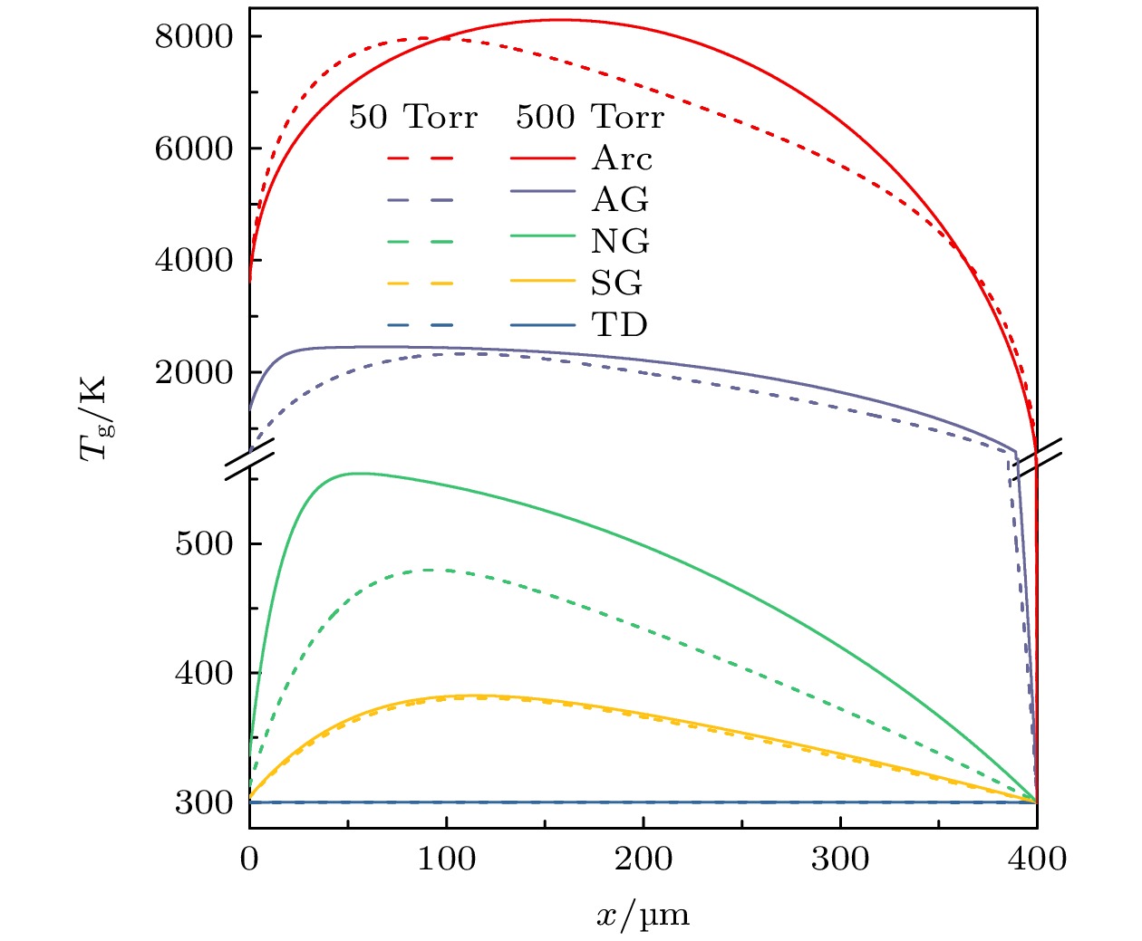
图 12 p = 50, 500 Torr气压条件下, 不同放电模式气体温度的空间分布

Fig. 12. Spatial distributions of gas temperature in different discharge regimes at $p=50,500 \;\text{Torr}$.

下载: 全尺寸图片幻灯片

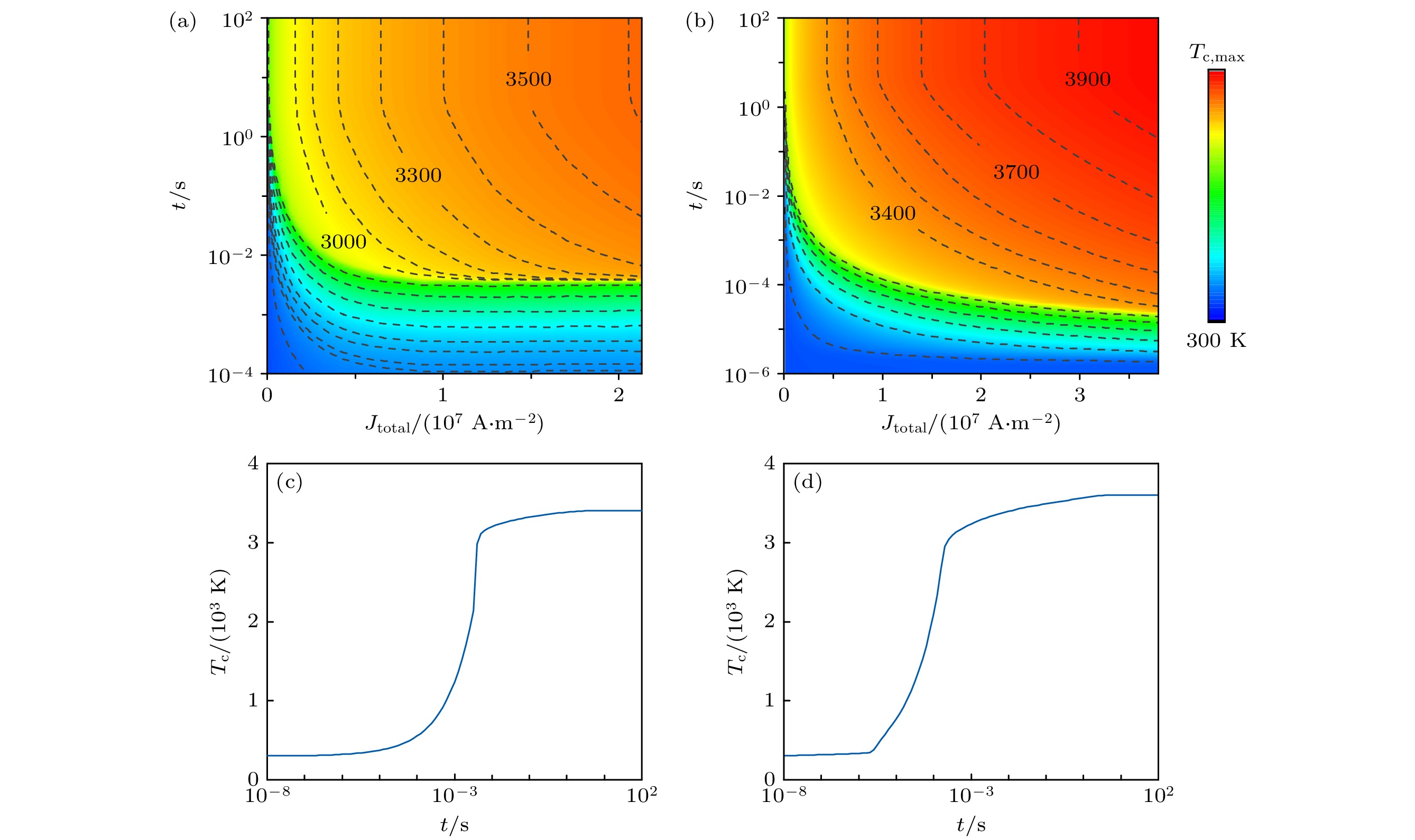
图 13 (a) $p_1 = 50 \;\text{Torr}$与(b) $p_2 = 500 \;\text{Torr}$时不同电流密度下阴极表面温度随时间的演化. 初始温度为300 K. 500 Torr时, 阴极表面温度最大值为$T_\text{c,max} = 3961 \;\text{K}$. 电流密度为$1 \times 10^7 \;\text{A}/\text{m}^2$时(c) $p_1 = 50 \;\text{Torr}$与(d) $p_2 = 500 \;\text{Torr}$条件下阴极表面温度随时间的变化

Fig. 13. Evolution of cathode surface temperature scaling with current density at (a) 50 Torr and (b) 500 Torr. The initial temperature is 300 K. The maxmium cathode surface temperature ($ T_\text{c,max}$) is 3961 K at 500 Torr. The temperature of cathode surface scaling with time when the current density is $J_\text{total} = 1 \times 10^7 \;\text{A}/\text{m}^2$ at (c) 50 Torr and (d) 500 Torr.

下载: 全尺寸图片幻灯片

表 1 该模型中计算的等离子体化学反应

Table 1. Reactions involved in the model

序号	反应过程	反应系数	参考文献	$\Delta E$/eV^[41]
R1	e + Ar $\rightarrow $ e + Ar	BOLSIG+	[47]	0
R2	e + Ar $\rightarrow $ e + $\text{Ar}^*$	BOLSIG+	[47]	11.5
R3	e + $\text{Ar}^*$ $\rightarrow $ e + Ar	BOLSIG+	[47]	–11.5
R4	e + Ar $\rightarrow $ 2e + $\text{Ar}^+$	BOLSIG+	[47]	15.8
R5	e + $\text{Ar}^*$ $\rightarrow $ 2e + $\text{Ar}^+$	BOLSIG+	[47]	4.3
R6	e + $\text{Ar}_2^*$ $\rightarrow $ 2e + $\text{Ar}_2^+$	BOLSIG+	[47]	3.66
R7	e + $\text{Ar}_2^*$ $\rightarrow $ e + 2Ar	BOLSIG+	[47]	–11.27
R8	e + $\text{Ar}_2^+$ $\rightarrow $ $\text{Ar}^*$ + Ar	$ 1.04\times {{10}^{-12}} {(0.026/{T_\text{e})}^{0.67}}\dfrac{1-\exp (-418/{T_\text{g}})}{1-0.31\exp (-418/{T_\text{g}})} \; [\text{m}^3/\text{s}] $	[48]	–3.03
R9	e + $\text{Ar}_2^+$ $\rightarrow $ e + $\text{Ar}^+$ + Ar	$ 1.11\times {{10}^{-12}}{{T}_\text{e}^{-1}}{\exp \{-[2.94+3({T_\text{g}}/11600-0.026)]\}}\; [\text{m}^3/\text{s}] $	[49,50]	4.53
R10	2e + $\text{Ar}^+$ $\rightarrow $ e + Ar	$ \left\{ \begin{array}{l}8.75 \times 10^{-39} T_\text{e}^{-4.5}\;[\text{m}^6/\text{s}], \; T_\text{e} \leqslant 0.276 \;\text{eV}\\1.29 \times 10^{-44}\left({11.659}/{T_{\mathrm{e}}}+2\right) \exp \left({4.11}/{T_\text{e}}\right)\;[\text{m}^6/\text{s}], \; T_\text{e} > 0.276 \;\text{eV}\end{array}\right. $	[50]	–15.8
R11	$\text{Ar}^$ + $\text{Ar}^$ $\rightarrow $ e + $\text{Ar}^+$ + Ar	$ 1.62\times {{10}^{-16}}{{T_\text{g}}^{0.5}} \; [\text{m}^3/\text{s}] $	[51]	–13.26
R12	$\text{Ar}^*$ + Ar $\rightarrow $ Ar + Ar	$ 3\times {{10}^{-21}}\; [\text{m}^3/\text{s}] $	[52,53]	–11.5
R13	2$\text{Ar}_2^*$ $\rightarrow $ e + 2Ar + $\text{Ar}_2^+$	$ 1.6248\times {{10}^{-16}}{{T_\text{g}}^{0.5}}\; [\text{m}^3/\text{s}] $	[54]	–8.01
R14	2Ar + $\text{Ar}^+$ $\rightarrow $ Ar + $\text{Ar}_2^+$	$ 7.5\times {{10}^{-41}}/T_\text{g} \; [\text{m}^6/\text{s}] $	[54]	–1.27
R15	2Ar + $\text{Ar}^$ $\rightarrow $ Ar + $\text{Ar}_2^$	$ 3.3\times {{10}^{-44}}\; [\text{m}^6/\text{s}] $	[39]	–0.23
R16	Ar + $\text{Ar}_2^+$ $\rightarrow $ 2Ar + $\text{Ar}^+$	$ 6.06\times {{10}^{-12}}{T_\text{g}^{-1}}{\exp (-1.258\times {{10}^{5}}/{{R}_{\text{g}}}/{T_\text{g}})}\; [\text{m}^3/\text{s}] $	[49,50]	1.27
R17	$\text{Ar}^*$ $\rightarrow $ Ar + $h\nu$	$ 3.145\times {{10}^{5}}\; [1/\text{s}] $	[55]	–11.5
R18	$\text{Ar}_2^*$ $\rightarrow $ 2Ar + $h\nu$	$ 6.00\times {{10}^{7}} \; [1/\text{s}] $	[39]	–11.27

下载: 导出CSV

表 2 p = 50, 500 Torr时反常辉光放电区电场反转、离子密度最大值、电势最大值、电子扩散电流密度与总电子电流密度相等、离子电流密度为零值的位置

Table 2. Position where the electric field is reversed ($x_{\text{r}}$), the ion density is maximum ($x_{\text{i}_\text{max}}$), the electric potential is maximum ($x_{\phi _ \text{max}}$), the electron diffusion current density equals the total electron current density ($x_{J_\text{e,dif}=J_\text{e}}$), and the ion current density equals zero ($x_{J_\text{i} = 0}$) at 50 Torr and 500 Torr in abnormal glow regime.

p/Torr	$x_{\text{r}}/\text{μm}$	$x_{\text{i}_\text{max}}/\text{μm}$	$x_{\phi _ \text{max}}/\text{μm}$	$x_{J_\text{e,dif}=J_\text{e}}/\text{μm}$	$x_{J_\text{i} = 0}/\text{μm}$
50	305.7	305.1	305.7	305.8	305.7
500	183.1	179.6	183.1	181.4	183.1

下载: 导出CSV

[1]	Hara K, Hanquist K 2018 Plasma Sources Sci. Technol. 27 065004 Google Scholar
[2]	Campanell M D, Johnson G R 2019 Phys. Rev. Lett. 122 015003 Google Scholar
[3]	Nanbu K 1980 J. Phys. Soc. Jpn. 49 2042 Google Scholar
[4]	Wilczek S, Schulze J, Brinkmann R P, Donkó Z, Trieschmann J, Mussenbrock T 2020 J. Appl. Phys. 127 181101 Google Scholar
[5]	Donkó Z, Derzsi A, Vass M, Horváth B, Wilczek S, Hartmann B, Hartmann P 2021 Plasma Sources Sci. Technol. 30 095017 Google Scholar
[6]	Petrović Z L, Škoro N, Marić D, Mahony C M O, Maguire P D, Radmilović-Rađenović M, Malović G 2008 J. Phys. D: Appl. Phys. 41 194002 Google Scholar
[7]	Yang D, Wang H H, Zheng B C, Zou X B, Wang X X, Fu Y Y 2023 Phys. Plasmas 30 063510 Google Scholar
[8]	Yang D, Wang H H, Zheng B C, Liu Z G, Fu Y Y 2023 Plasma Sources Sci. Technol. 32 10LT01 Google Scholar
[9]	付洋洋, 罗海云, 邹晓兵, 王强, 王新新 2014 物理学报 63 095206 Google Scholar Fu Y Y, Luo H Y, Zou X B, Wang Q, Wang X X 2014 Acta Phys. Sin. 63 095206 Google Scholar
[10]	Zhao Z H, Wei X L, Guan R Y, Nie H Y, Zhu B, Yao Y H 2022 IEEE Trans. Plasma Sci. 50 2333 Google Scholar
[11]	张晓宁, 李和平, Murphy A B, 夏维生 2013 高电压技术 39 7 Google Scholar Zhang X N, Li H P, Murphy A B, Xia W S 2013 High Voltage Eng. 39 7 Google Scholar
[12]	Surendra M, Graves D B, Jellum G M 1990 Phys. Rev. A 41 1112 Google Scholar
[13]	Fiala A, Pitchford L C, Boeuf J P 1994 Phys. Rev. E 49 5607 Google Scholar
[14]	Farouk T, Farouk B, Staack D, Gutsol A, Fridman A 2006 Plasma Sources Sci. Technol. 15 676 Google Scholar
[15]	Bogaerts A, Gijbels R, Goedheer W J 1996 Anal. Chem. 68 2296 Google Scholar
[16]	Liu X H, He W, Yang F, Wang H Y, Liao R J, Xiao H G 2012 Chin. Phys. B 21 075201 Google Scholar
[17]	Chen S, Nobelen J, Nijdam S 2017 Plasma Sources Sci. Technol. 26 095005 Google Scholar
[18]	Chen S, Li K, Nijdam S 2019 Plasma Sources Sci. Technol. 28 055017 Google Scholar
[19]	Wang L, Chen S, Wang F 2019 Plasma Chem. Plasma Process. 39 1291 Google Scholar
[20]	Liu F C, Guo X, Zhou Z X, He Y F, Fan W L 2019 Phys. Plasmas 26 123505 Google Scholar
[21]	Marić D, Hartmann P, Malović G, Donkó Z, Petrović Z L 2003 J. Phys. D: Appl. Phys. 36 2639 Google Scholar
[22]	Zhu Y F, Starikovskaia S 2018 Plasma Sources Sci. Technol. 27 124007 Google Scholar
[23]	Wu Y, Zhu Y F, Cui W, Jia M, Li Y H 2015 Plasma Processes Polym. 12 642 Google Scholar
[24]	Chen X C, Zhu Y F, Wu Y, Su Z, Liang H 2020 Plasma Processes Polym. 53 465202 Google Scholar
[25]	Babaeva N Y, Kushner M J 2009 J. Phys. D: Appl. Phys. 42 132003 Google Scholar
[26]	Babaeva N Y, Naidis G V 2016 Phys. Plasmas 23 083527 Google Scholar
[27]	Nijdam S, Teunissen J, Ebert U 2020 Plasma Sources Sci. Technol. 29 103001 Google Scholar
[28]	Luque A, Ratushnaya V, Ebert U 2008 J. Phys. D: Appl. Phys. 41 234005 Google Scholar
[29]	Yan W, Economou D J 2017 J. Phys. D: Appl. Phys. 50 415205 Google Scholar
[30]	Jiang Y Y, Wang Y H, Zhang J, Wang D Z 2022 J. Phys. D: Appl. Phys. 55 335203 Google Scholar
[31]	Kolobov V I, Fiala A 1994 Phys. Rev. E 50 3018 Google Scholar
[32]	Arslanbekov R R, Kolobov V I 2003 J. Phys. D: Appl. Phys. 36 2986 Google Scholar
[33]	Eliseev S I, Kudryavtsev A A, Liu H, Ning Z X, Yu D R, Chirtsov A S 2016 IEEE Trans. Plasma Sci. 44 2536 Google Scholar
[34]	Fu Y Y, Zhang P, Verboncoeur J P 2018 Appl. Phys. Lett. 112 254102 Google Scholar
[35]	Fu Y Y, Zhang P, Krek J, Verboncoeur J P 2019 Appl. Phys. Lett. 114 014102 Google Scholar
[36]	Fu Y Y, Wang H H, Zheng B C, Zhang P, Fan Q H, Wang X X, Verboncoeur J P 2021 Appl. Phys. Lett. 118 401 Google Scholar
[37]	Fu Y Y, Krek J, Zhang P, Verboncoeur J P 2018 IEEE Trans. Plasma Sci. 47 2011 Google Scholar
[38]	Chen J D, Verboncoeur J P, Fu Y Y 2022 Appl. Phys. Lett. 121 074102 Google Scholar
[39]	Baeva M, Loffhagen D, Uhrlandt D 2019 Plasma Chem. Plasma Process. 39 1359 Google Scholar
[40]	Baeva M, Loffhagen D, Becker M M, Uhrlandt D 2019 Plasma Chem. Plasma Process. 39 949 Google Scholar
[41]	Baeva M, Uhrlandt D, Loffhagen D 2020 Jpn. J. Appl. Phys. 59 SHHC05 Google Scholar
[42]	Saifutdinov A I, Fairushin I I, Kashapov N F 2016 JETP Lett. 104 180 Google Scholar
[43]	Saifutdinov A I 2021 J. Appl. Phys. 129 093302 Google Scholar
[44]	Saifutdinov A I 2022 Plasma Sources Sci. Technol. 31 094008 Google Scholar
[45]	王大智, 袁博文, 卢琪, 乔俊杰, 熊青 2023 电工技术学报 38 09 Google Scholar Wang D Z, Yuan B W, Lu Q, Qiao J J, Xiong Q 2023 Trans. China Electrotech. Soc. 38 09 Google Scholar
[46]	Bogaerts A, Gijbels R 1999 J. Appl. Phys. 86 4124 Google Scholar
[47]	Hayashi M 2003 Bibliography of Electron and Photon Cross Sections with Atoms and Molecules published in the 20th century (Toki, Gifu: National Inst. for Fusion Science) NIFS-DATA-72
[48]	Cunningham A J, O’Malley T F, M H R 1981 J. Phys. B: At. Mol. Phys. 14 773 Google Scholar
[49]	Jonkers J, Sande M van de, Sola A, Gamero A, Rodero A, Mullen J van der 2003 Plasma Sources Sci. Technol. 12 464 Google Scholar
[50]	Niu C, Hu Y H, Shao K, Sun S R, Wang H X 2022 Plasma Chem. Plasma Process. 42 885 Google Scholar
[51]	Kolokolov N B, Kudrjavtsev A A, Blagoev A B 1994 Phys. Scr. 50 371 Google Scholar
[52]	Lymberopoulos D P, Economou D J 1993 J. Appl. Phys. 73 3668 Google Scholar
[53]	Karoulina E V, Lebedev Y A 1992 J. Phys. D: Appl. Phys. 25 401 Google Scholar
[54]	Kannari F, Suda A, Obara M, Fujioka T 1983 IEEE J. Quantum Electron. 19 1587 Google Scholar
[55]	Gregório J, Leprince P, Boisse-Laporte C, Alves L L 2012 Plasma Sources Sci. Technol. 21 015013 Google Scholar
[56]	Rafatov I, Bogdanov E A, Kudryavtsev A A 2012 Phys. Plasmas 19 033502 Google Scholar
[57]	Kolokolov N B, Blagoev A B 1993 Phys.-Usp. 36 152 Google Scholar
[58]	Beulens J J, Milojevic D, Schram D C, Vallinga P M 1991 Phys. Fluids B 3 2548 Google Scholar
[59]	杜世刚 1998 等离子体物理 (北京: 原子能出版社) 第160—163页 Du S G 1998 Plasma Physics (Beijing: Atomic Press) pp160–163
[60]	Bird R B, Steward W E, Lightfoot E N 2001 Transport Phenomena (Hoboken: Wiley) p526
[61]	Chapman S, Cowling T G 1995 The Mathematical Theory of Non-uniform Gases: an Account of the Kinetic Theory of Viscosity, Thermal Conduction and Diffusion in Gases (Cambridge: Cambridge university Press) p167
[62]	张东荷雨, 刘金宝, 付洋洋 2024 物理学报 73 025201 Google Scholar Zhang D H Y, Liu J B, Fu Y Y 2024 Acta Phys. Sin. 73 025201 Google Scholar
[63]	Brokaw R S 1969 Ind. Eng. Chem. Process Des. Dev. 8 240 Google Scholar
[64]	Neufeld P D, Janzen A R, Aziz R A 1972 J. Chem. Phys. 57 1100 Google Scholar
[65]	Gurvich L V, Veyts I V, Alcock C B 1989 Thermodynamic Properties of Individual Substances (Vol. 1) (4th Ed.) (Washington: Hemisphere Publishing Corp) pp135–138
[66]	Maltsev M A, Morozov I V, Osina E L 2019 High Temp. 57 37 Google Scholar
[67]	刘富成, 晏雯, 王德真 2013 物理学报 62 175204 Google Scholar Liu F C, Yan W, Wang D Z 2013 Acta Phys. Sin. 62 175204 Google Scholar
[68]	Incropera F P, DeWitt D P, Bergmann T L, Lavine A S 2007 Fundamentals of Heat and Mass Transfer (New York: John Wiley) p68
[69]	Touloukian Y S, Powell R W, Ho C Y, Clemens P G 1970 Thermal Conductivity: Metallic Tlements and Alloys (Thermophysical Properties of Matter) (New York: Plenum Press) pp415−428
[70]	Brown S B 1959 Basic Data of Plasma Physics (New York: John Wiley and Sons, Inc.) pp167–211
[71]	Schottky W 1914 Ann. Phys. 44 1011 Google Scholar
[72]	杨津基 1983 气体放电 (北京: 科学出版社) 第50页 Yang J J 1983 Gas Discharge (Beijing: Science Press) p50
[73]	邵先军, 马跃, 李娅西, 张冠军 2010 物理学报 59 8747 Google Scholar Shao X J, Ma Y, Li Y X, Zhang G J 2010 Acta Phys. Sin. 59 8747 Google Scholar
[74]	COMSOL AB, Stockholm, Sweden COMSOL Multiphysics^® v.6.1
[75]	Si Ma W X, Peng Q J, Yang Q, Yuan T, Shi J 2012 IEEE Trans. Dielectr. Electr. Insul. 19 660 Google Scholar
[76]	Zhuang Y, Chen G, Rotaru M 2011 J. Phys: Conference Series 310 012011 Google Scholar
[77]	Raizer Y P 1991 Gas Discharge Physics (Berlin: Springer-Verlag) pp167–211
[78]	Gudmundsson J T, Hecimovic A 2017 Plasma Sources Sci. Technol. 26 123001 Google Scholar
[79]	Paschen F 1889 Ann. Phys. 273 69 Google Scholar
[80]	徐学基, 诸定昌 1996 气体放电物理 (上海: 复旦大学出版社) 第121—126页 Xu X J, Zhu D C 1996 Gas Discharge Physics (Shanghai: Fudan University Press) pp121–126
[81]	Townsend J S 1900 Nature 62 340 Google Scholar
[82]	岳清宇, 金花 1988 辐射防护 6 1 Yue Q Y, Jin H 1988 Radiat. Prot. 6 1
[83]	Lü B, Wang X X, Luo H Y, Liang Z 2009 Chin. Phys. B 18 646 Google Scholar
[84]	梁曦东, 周远翔, 曾嵘 2015 高电压工程(第2版) (北京: 清华大学出版社) 第17, 18页 Liang X D, Zhou Y X, Zeng R 2015 High Voltage Engineering (2nd Ed.) (Beijing: Tsinghua University Press) pp17, 18
[85]	Bouchikhi A, Hamid A 2010 Plasma Sci. Technol. 12 59 Google Scholar
[86]	Levko D, Subramaniam V, Raja L L 2022 Phys. Plasmas 29 023503 Google Scholar
[87]	Bogaerts A, Neyts E, Gijbels R, Van der M J 2002 Spectrochim. Acta, Part B 57 609 Google Scholar
[88]	Bogaerts A, Gijbels R, Goedheer W J 1995 J. Appl. Phys. 78 2233 Google Scholar
[89]	姚聪伟, 马恒驰, 常正实, 李平, 穆海宝, 张冠军 2017 物理学报 66 025203 Google Scholar Yao C W, Ma H C, Chang Z S, Li P, Mu H B, Zhang G J 2017 Acta Phys. Sin. 66 025203 Google Scholar
[90]	Montie T C, Kelly-Wintenberg K, Roth J R 2000 IEEE Trans. Plasma Sci. 28 41 Google Scholar
[91]	Gottscho R A, Mitchell A, Scheller G R, Chan Y Y, Graves D B 1989 Phys. Rev. A 40 6407 Google Scholar
[92]	Wang Q, Economou D J, Donnelly V M 2006 J. Appl. Phys. 100 023301 Google Scholar
[93]	Kolobov V I, Tsendin L D 1992 Phys. Rev. A 46 7837 Google Scholar
[94]	Boeuf J P, Pitchford L C 1995 J. Phys. D: Appl. Phys. 28 2083 Google Scholar
[95]	Kudryavtsev A A, Toinova N E 2005 Tech. Phys. Lett. 31 370 Google Scholar
[96]	Kudryavtsev A A, Nisimov S U, Prokhorova E I, Slyshov A G 2011 Tech. Phys. Lett. 37 838 Google Scholar
[97]	Kudryavtsev A A, Nisimov S U, Prokhorova E I, Slyshov A G 2012 Tech. Phys. 57 1188 Google Scholar
[98]	Barzilovich K A, Bogdanov E A, Kudryavtsev A A 2014 Tech. Phys. Lett. 40 581 Google Scholar
[99]	Marić D, Kutasi K, Malović G, Petrović Z L 2002 Eur. Phys. J. D 21 73 Google Scholar
[100]	Phelps A V 2001 Plasma Sources Sci. Technol. 10 329 Google Scholar
[101]	Franklin R N 2003 J. Phys. D: Appl. Phys. 36 R309 Google Scholar

[1]	朱海龙, 师玉军, 王嘉伟, 张志凌, 高一宁, 张丰博. 高气压氩气辉光放电条纹等离子体的形成和演化. 物理学报, 2022, 71(14): 145201. doi: 10.7498/aps.71.20212394
[2]	郑建东, 周江, 皮晓丽, 邹晨, 李一帆, 徐坤博, 龚自正, 胡帼杰. 空间碎片超高速撞击下太阳电池阵伏安特性. 物理学报, 2021, 70(18): 188801. doi: 10.7498/aps.70.20210458
[3]	李雪辰, 耿金伶, 贾鹏英, 吴凯玥, 贾博宇, 康鹏程. 液体电极上辉光放电丝的运动特性研究. 物理学报, 2018, 67(7): 075201. doi: 10.7498/aps.67.20172205
[4]	侯兴民, 章程, 邱锦涛, 顾建伟, 王瑞雪, 邵涛. 大气压管板结构纳秒脉冲放电中时域X射线研究. 物理学报, 2017, 66(10): 105204. doi: 10.7498/aps.66.105204
[5]	姚聪伟, 马恒驰, 常正实, 李平, 穆海宝, 张冠军. 大气压介质阻挡辉光放电脉冲的阴极位降区特性及其影响因素的数值仿真. 物理学报, 2017, 66(2): 025203. doi: 10.7498/aps.66.025203
[6]	白占国, 李新政, 李燕, 赵昆. 气体放电系统中多臂螺旋波的数值分析. 物理学报, 2014, 63(22): 228201. doi: 10.7498/aps.63.228201
[7]	章程, 马浩, 邵涛, 谢庆, 杨文晋, 严萍. 纳秒脉冲气体放电中逃逸电子束流的研究. 物理学报, 2014, 63(8): 085208. doi: 10.7498/aps.63.085208
[8]	付洋洋, 罗海云, 邹晓兵, 王强, 王新新. 棒-板电极下缩比气隙辉光放电相似性的仿真研究. 物理学报, 2014, 63(9): 095206. doi: 10.7498/aps.63.095206
[9]	付洋洋, 罗海云, 邹晓兵, 刘凯, 王新新. 缩比间隙中辉光放电相似性的初步研究. 物理学报, 2013, 62(20): 205209. doi: 10.7498/aps.62.205209
[10]	胡明, 万树德, 钟雷, 刘昊, 汪海. 磁控直流辉光等离子体放电特性. 物理学报, 2012, 61(4): 045201. doi: 10.7498/aps.61.045201
[11]	俞哲, 张芝涛, 于清旋, 许少杰, 姚京, 白敏冬, 田一平, 刘开颖. 针-板DBD微流注与微辉光交替生成的机理研究. 物理学报, 2012, 61(19): 195202. doi: 10.7498/aps.61.195202
[12]	贺亚峰, 冯晓敏, 张亮. 气体放电系统中时空斑图的时滞反馈控制. 物理学报, 2012, 61(24): 245204. doi: 10.7498/aps.61.245204
[13]	武晋泽, 唐晋娥, 董有尔, 张国峰, 王彦华. 常压下气体放电等离子体振荡的实验与理论研究. 物理学报, 2012, 61(19): 195208. doi: 10.7498/aps.61.195208
[14]	章程, 邵涛, 牛铮, 张东东, 王珏, 严萍. 大气压尖板电极结构重复频率纳秒脉冲放电中X射线辐射特性研究. 物理学报, 2012, 61(3): 035202. doi: 10.7498/aps.61.035202
[15]	沈向前, 谢泉, 肖清泉, 陈茜, 丰云. 磁控溅射辉光放电特性的模拟研究. 物理学报, 2012, 61(16): 165101. doi: 10.7498/aps.61.165101
[16]	李英德, 李宗良, 冷建材, 李伟, 王传奎. 光致异构体开关特性的理论研究. 物理学报, 2011, 60(7): 073101. doi: 10.7498/aps.60.073101
[17]	马松山, 朱佳, 徐慧, 郭锐. 碱基对组分、电极位能及界面耦合对DNA分子I-V特性的影响. 物理学报, 2010, 59(10): 7458-7462. doi: 10.7498/aps.59.7458
[18]	张燕, 顾彪, 王文春, 彭许文, 王德真. 常压He气和N2气均匀介质阻挡放电的伏安特性. 物理学报, 2009, 58(8): 5532-5538. doi: 10.7498/aps.58.5532
[19]	马勇, 邹斌, 李宗良, 王传奎, 罗毅. 六元杂环分子电学特性的理论研究. 物理学报, 2006, 55(4): 1974-1978. doi: 10.7498/aps.55.1974
[20]	王建华, 金传恩. 蒙特卡罗模拟在辉光放电鞘层离子输运研究中的应用. 物理学报, 2004, 53(4): 1116-1122. doi: 10.7498/aps.53.1116

计量

文章访问数: 3934
PDF下载量: 150
被引次数: 0

姓名
邮箱
手机号码
标题
留言内容
验证码

搜索

留言板